All-NVMe Ceph for AI: When Distributed Storage Actually Beats Local ZFS

There is a belief in infrastructure circles that refuses to die:

“Nothing beats local NVMe.”

And for a single box running a transactional database, that’s mostly true. If you are minimizing latency for a single SQL instance, keep your storage close to the CPU.

But AI clusters aren’t single boxes. And as we detailed in The Storage Wall: ZFS vs. Ceph vs. NVMe-oF, once you reach the petabyte scale, “latency” stops being your primary metric during the training read phase.

AI training is synchronized, parallel, and massive. The bottleneck isn’t nanosecond-level latency anymore. It is aggregate throughput under parallel pressure.

That is where an All-NVMe deployment of Ceph—even using Erasure Coding (EC) 6+2 – can outperform mirrored local ZFS. Not because it’s “faster” on a spec sheet.

Because it scales during dataset distribution.

This becomes the dominant physics reality once the dataset no longer fits comfortably inside a single node’s working set. Below that threshold, local NVMe still wins. Above it, the problem stops being storage latency and becomes synchronization bandwidth.

(Note: The inverse problem—extremely latency-sensitive checkpoint writes – is where NVMe-oF still dominates, a distinction we cover separately in our checkpoint stall analysis.)

That crossover point is usually reached long before teams expect it—often when dataset size exceeds the aggregate ARC + Page Cache of a node rather than the raw capacity of the disks.

The Symptom Nobody Attributes to Storage

The first sign this problem exists usually isn’t a disk alert. It’s this:

Your training job runs fine for the first few minutes. Then, at the start of every epoch, throughput collapses.

• GPU utilization drops from 95% to 40%.
• CPU usage spikes in kworker.
• Disks show 100% busy — but only on some nodes.

You restart the job and it improves for exactly one epoch. So you blame the framework. You blame the scheduler.

But what’s actually happening is synchronized dataset re-reads.

Each node is independently saturating its own local storage while the rest of the cluster waits at a barrier. The GPUs aren’t slow. They’re waiting for data alignment across workers.

The Lie We Tell Ourselves About Local NVMe

A modern AI training node is a beast. On paper, it looks perfect:

• 2–4 Gen4/Gen5 NVMe drives
• ZFS mirror or stripe
• 6–12 GB/s sequential read per node
• Sub-millisecond latency

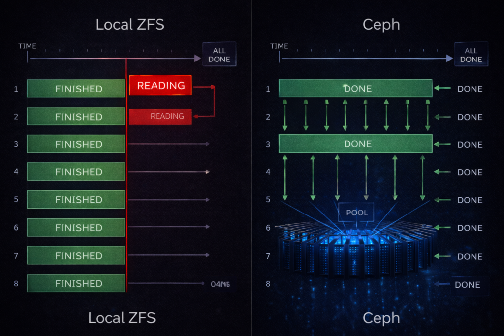
On a whiteboard, that architecture is beautiful. But now, multiply it.

Take that single node and scale it to an 8-node cluster with 64 GPUs, crunching a 200 TB training dataset. Suddenly, you don’t have one fast storage system.

You have eight isolated islands.

Local storage scales per node.

AI training scales per barrier.

That architectural mismatch is the silent killer of GPU efficiency. Barrier synchronization is the heartbeat of distributed training; if one node misses a beat, the whole cluster pauses.

Why AI Workloads Break “Local Is Best”

Deep learning frameworks like PyTorch and TensorFlow do not behave like OLTP databases. Their I/O patterns are hostile to traditional storage logic:

1. Streaming Shards: Massive sequential reads.
2. Parallel Workers: Multiple loaders per GPU.
3. Epoch Cycling: Full dataset re-reads.
4. The “Read Storm”: Every GPU demands data simultaneously.

The most misleading metric in AI storage is average throughput. What matters is synchronized throughput at barrier time.

With local ZFS, you are forced into duplicate datasets or caching gymnastics that collapse under scale. Neither is elegant at 100TB+.

The All-NVMe Ceph Pattern That Works

In production GPU clusters, the architecture that consistently delivers saturation-level throughput during training reads looks like this:

• 6–12 Dedicated Storage Nodes (separate from compute)
• NVMe-only OSDs
• 100/200GbE Fabric (non-blocking spine-leaf)
• BlueStore Backend
• EC 6+2 Pool for large datasets

The goal here is not latency dominance. The goal is aggregate cluster bandwidth.

If you have eight storage nodes capable of delivering 3 GB/s each, you don’t care about the 3 GB/s. You care about the 24 GB/s shared across the cluster simultaneously—shared, striped, and resilient.

Sanity Check Your Architecture Instead of guessing whether your fabric can handle the read storm, I built a tool to model it. You can input your exact GPU count, dataset size, and network speed to see if your current design will hit a synchronization wall.

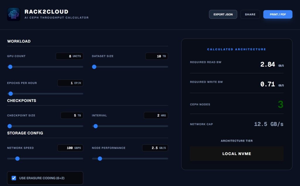
Run the AI Ceph Throughput Calculator:

If the calculator shows your “Required Read BW” exceeding your network cap, adding more local NVMe won’t save you. You need to widen the pipe.

Real Benchmark Methodology (Not Marketing Slides)

If we want to move this from opinion to authority, we need methodology.

The Local ZFS Test (Per Node)

Running a standard fio test on a local Gen4 mirror:

Bash

fio --name=seqread \
    --filename=/tank/testfile \
    --rw=read \
    --bs=1M \
    --iodepth=32 \
    --numjobs=8 \
    --size=100G \
    --direct=1 \
    --runtime=120 \
    --group_reporting

Typical Result: You see a strong 7–9 GB/s read. Ideally, this looks great. But across 8 nodes, you don’t get a unified 64 GB/s throughput pool. You get 8 independent pipes.

The Ceph EC 6+2 Test

• Infrastructure: 8 OSD Nodes, 4 NVMe per node, 100GbE fabric.
• Profile: Erasure Code 6+2 (6 data chunks, 2 parity).

Step 1: Create the Profile

Bash

ceph osd erasure-code-profile set ec-6-2 \
    k=6 m=2 \
    crush-failure-domain=host \
    crush-device-class=nvme

Step 2: Tune BlueStore (ceph.conf) Defaults won’t cut it for high-throughput AI.

Ini, TOML

[osd]
osd_memory_target = 8G
bluestore_cache_size = 4G
bluestore_min_alloc_size = 65536
osd_op_num_threads_per_shard = 2
osd_op_num_shards = 8

The Reality: Per OSD node, you might only see 2–4 GB/s. But across the cluster? You are seeing 20–30+ GB/s of aggregate, sustained read throughput. The GPUs are no longer fighting per-node silos. They are pulling from a massive, shared bandwidth fabric.

The EC 6+2 Performance Reality

Yes, erasure coding adds a write penalty. But training datasets are read-dominant once staged.

(Checkpoint write bursts remain a separate storage class problem—typically solved with a low-latency tier such as NVMe-oF.)

With large object sizes (≥1MB), EC read amplification is negligible compared to dataset parallelism overhead.

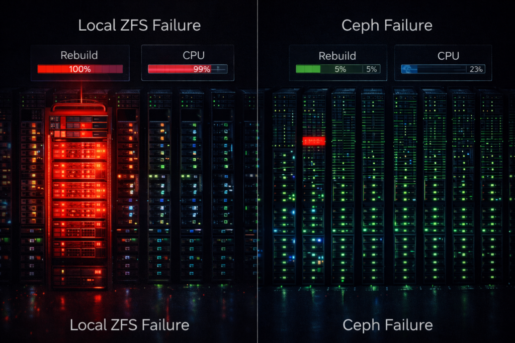
Why Rebuild Behavior Matters More Than Latency

Benchmarks happen on healthy systems. Training happens on degraded ones.

In a mirrored local ZFS layout, a single NVMe failure turns one node into a rebuild engine. The controller saturates, latency spikes, and that node misses synchronization barriers.

The entire training job slows to the speed of the worst node.

Ceph distributes reconstruction across the cluster. No node becomes the designated victim. Your training run continues at ~85% speed instead of collapsing.

Capacity Math at Scale

Finally, let’s talk about the budget.

• Local Mirror: 50% usable capacity.
• Ceph EC 6+2: 75% usable capacity.

At 500TB scale, that 25% delta funds additional GPUs. More importantly, it creates architectural separation:

1. Ceph: Training dataset distribution.
2. Low-Latency Tier: Checkpoint persistence.
3. Vault Storage: Immutable backups.

Each layer solves a different failure mode.

The Architect’s Verdict

Eventually every AI cluster discovers the same thing:

Storage stops being about speed. It becomes about coordination.

Local NVMe optimizes individual nodes. Distributed training punishes individual optimization. All-NVMe Ceph isn’t the lowest latency storage. It’s the storage that keeps the entire cluster moving at once.

And once datasets exceed the working memory of a node, synchronized movement beats isolated speed.

This article is part of our AI Infrastructure Pillar. If you are currently designing your data pipeline, we recommend continuing with the Storage Architecture Learning Path, where we break down the specific tuning required for BlueStore NVMe backends.

Additional Resources

• Ceph Erasure Coding Documentation
• PyTorch Data Loading Best Practices

About The Architect

R.M.

Senior Solutions Architect with 25+ years of experience in HCI, cloud strategy, and data resilience. As the lead behind Rack2Cloud, I focus on lab-verified guidance for complex enterprise transitions. View Credentials →