AI INFERENCE ARCHITECTURE
Cost Is Behavioral. Latency Is Physics. Neither Is Optional.
AI inference architecture is the layer of the AI infrastructure stack that most organizations get wrong first and most expensively. Not because the concepts are obscure, but because the mental models imported from adjacent infrastructure disciplines — application serving, cloud economics, batch processing — do not transfer. Inference does not behave like an application server under load. Its cost does not scale the way provisioned infrastructure costs scale. Its failure modes are not visible to the monitoring that works everywhere else in the stack. And the decisions made before the first model is deployed — silicon placement, serving architecture, concurrency budget, data gravity — are largely irreversible once production workloads are running against them.
The foundational distinction that governs AI inference architecture is one that traditional infrastructure practice has no direct equivalent for: inference economics are governed simultaneously by infrastructure physics and runtime behavior. Traditional infrastructure economics were governed primarily by utilization physics — provision the resource, pay for what you allocate, optimize through reservation and right-sizing. Inference economics are governed by both layers at once. The physics layer — latency, memory bandwidth, fabric constraints, concurrency stability — determines what the infrastructure is capable of. The behavioral layer — token consumption rates, retry frequency, agentic loop depth, retrieval amplification — determines what it actually costs to run. Both layers compound. Neither is optional. And most production AI teams are instrumented for one while flying blind on the other.
This page maps the full AI inference architecture across both governing domains: the four-layer Inference Architecture Stack from silicon through observability, the serving and concurrency physics that determine whether a production inference system is stable or fragile, the cost governance architecture that makes behavioral spend visible and controllable, the retrieval dynamics that change inference physics when RAG enters the stack, and the placement economics decision that determines where inference workloads belong as they stabilize and scale. The AI infrastructure stack context for where inference sits relative to training, fabric, and operations is the starting point for understanding why this layer requires its own architectural discipline.
What AI Inference Architecture Actually Is
Inference is the production phase of AI. Training produces the model. Inference is everything that happens after — every token generated, every request served, every API call answered, every agent action taken. It is the phase where AI infrastructure interacts with users, with downstream systems, and with the cost model that determines whether a production AI deployment is economically viable or quietly compounding toward a crisis.
AI inference architecture is the discipline of designing the infrastructure that governs that phase: the silicon it runs on, the serving runtime that processes requests, the concurrency model that determines stability under load, the cost governance layer that makes behavioral spend visible and controllable, and the placement decisions that determine where inference workloads live relative to the data, users, and systems they serve. It is distinct from training infrastructure — which is optimized for throughput saturation across a bounded, predictable workload — and distinct from the LLM operations control plane above it, which governs artifacts, lifecycle, and operational authority. Inference architecture governs the runtime infrastructure itself: what it is built from, how it behaves under load, and what it costs to operate.
The governing physics of inference differ from training in ways that make the mental model transfer dangerous. Training optimizes for a single metric — throughput, measured in tokens processed per second per GPU — across a workload class that is homogeneous (one job, one model, full cluster) and bounded (training ends, the cost event closes). Inference optimizes for two competing metrics simultaneously — Time to First Token for latency-sensitive workloads and throughput for cost efficiency — across a workload class that is heterogeneous (mixed request types, multiple concurrency levels, variable context lengths) and continuous (inference never ends; the cost event is open-ended and behavioral).
That simultaneity is the core challenge. Training infrastructure can be right-sized for a known throughput target. Inference infrastructure must be designed for a concurrency stability envelope — the range of request behavior within which the serving runtime maintains acceptable P99 latency — that shifts constantly as workload patterns evolve, models change, and retrieval systems alter the token economics of every request.
The two governing domains that structure this page and the discipline it covers:
Traditional infrastructure practice was almost entirely a physics discipline. You provisioned resources, measured utilization, and optimized through reservation and right-sizing. The behavioral layer barely existed — application code consumed the resources you provisioned, and the cost followed the provisioning. AI inference architecture requires governing both layers simultaneously. The physics determines the stability envelope. The behavior determines the cost inside it. Getting the physics right without governing the behavior produces an inference system that is stable and expensive. Getting the behavior right without designing the physics produces one that is cheap until it collapses under load. Most production failures involve both.
Why Inference Infrastructure Fails
Inference failures are not infrastructure outages. The hardware does not crash. The network does not partition. The failures are slower and more expensive: a serving stack that degrades silently under load, a cost model that compounds past every forecast, a concurrency envelope that collapses before hardware saturation gives any warning. The six failure modes below account for the majority of production inference incidents. Each maps to a specific gap in either the physics or behavioral governance layer.
The pattern across all six is consistent with the two-domain model: physics failures originate in infrastructure design decisions made before deployment, behavioral failures originate in runtime patterns that are invisible to infrastructure monitoring. The most expensive failures involve both — a physics constraint that triggers a behavioral response (Cold-Path Storm, where the autoscaling gap triggers retry amplification) or a behavioral pattern that exhausts a physical resource (Behavioral Cost Blindness, where token accumulation fills GPU memory). Neither layer governs the other. Both must be designed for simultaneously.
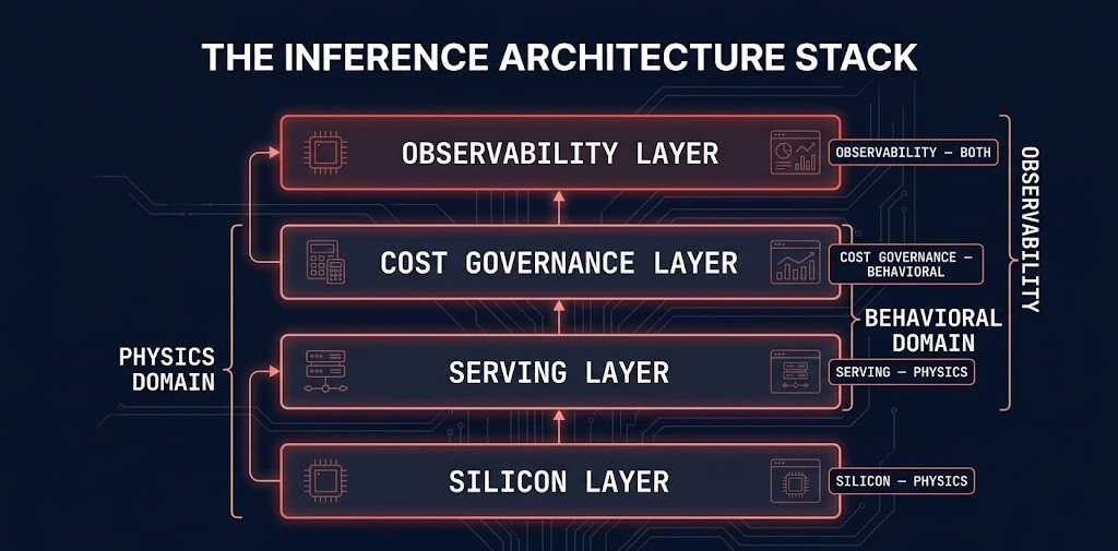
The Inference Architecture Stack
The Inference Architecture Stack is the four-layer model that structures AI inference infrastructure from the silicon that executes requests to the observability layer that makes runtime behavior visible. Each layer has distinct physics, distinct failure modes, and distinct governance requirements. Each layer depends on the one below it and exposes capabilities to the one above it. Optimizing any layer without understanding its dependencies produces local improvements and systemic vulnerabilities.
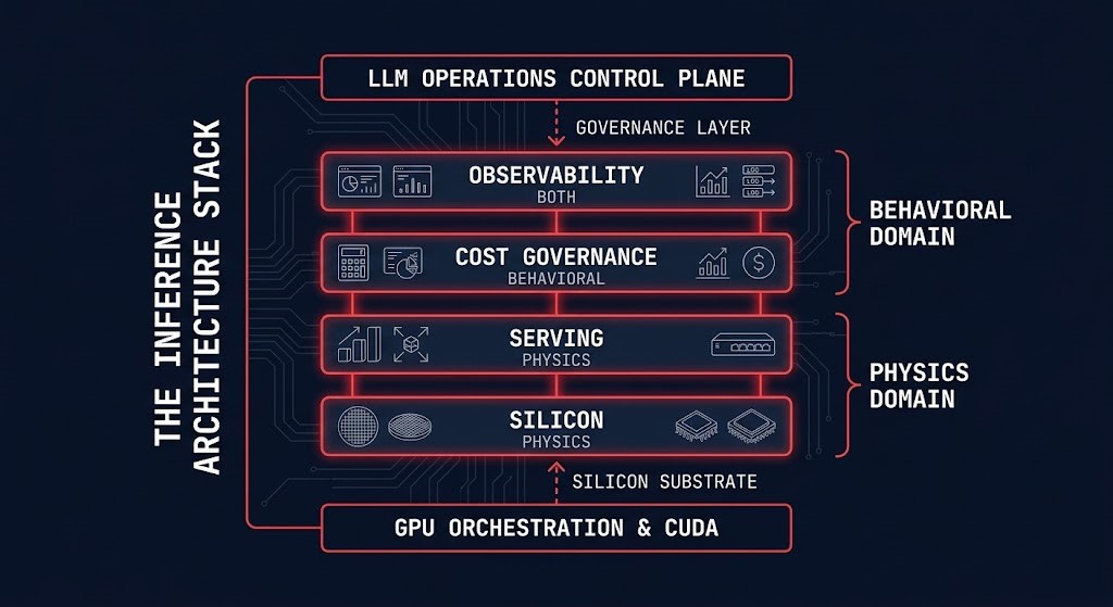
The stack’s relationship to the adjacent sub-pages is explicit by design. GPU Orchestration and CUDA governs the layer below the silicon — how accelerators are scheduled, partitioned, and isolated. The Inference Architecture Stack begins where GPU Orchestration ends: with the inference-specific decisions about what silicon to select, how to configure the serving runtime on top of it, how to govern the behavioral cost it produces, and how to instrument both domains in production. Above the stack, the LLM Operations Control Plane governs artifacts, versioning, rollback, and lifecycle — the operational discipline that makes the serving infrastructure deployable and maintainable. The stack is what is being governed. The control plane is what governs it.
The Distributed AI Fabrics architecture intersects at the silicon and serving layers — fabric P99 latency is a physics constraint that governs both distributed training synchronization and sharded inference serving. A sharded model deployment that hits fabric latency problems exhibits the same synchronization stall behavior as a distributed training job. The physics are the same. The operational context differs: in inference, the stall manifests as TTFT variance under load rather than gradient synchronization delay.
The Silicon Layer: Hardware Split and Workload Placement
The silicon layer is where inference architecture begins and where most teams make their first structural mistake. The mistake is not choosing wrong hardware — it is not choosing at all. Training infrastructure gets provisioned for training requirements, inference workloads get added to whatever silicon is available, and the mismatch between hardware optimization targets and workload requirements accumulates as idle cost, degraded latency, and a cost model that never closes.
The foundational design decision at the silicon layer is workload separation. Training and inference are not versions of the same computational problem. Training optimizes for sustained throughput across a homogeneous workload — maximize the gradient computation completed per second across a cluster where every node is running the same job. Inference optimizes for latency predictability and concurrency stability across a heterogeneous workload — maintain acceptable P99 TTFT across a continuous stream of requests that vary in length, context depth, and computational demand. The hardware characteristics that make a GPU excellent at training — high memory bandwidth for sequential matrix operations, large register files for gradient accumulation, NVLink optimization for all-reduce communication — are not the same characteristics that make silicon excellent at inference. Inference favors lower memory latency for KV cache access, higher memory capacity per compute unit for storing more concurrent sessions, and optimized attention kernels for the autoregressive token generation pattern that dominates inference compute.
GTC 2026 formalized this separation at the silicon level. For the first time, the industry shipped dedicated inference silicon — the Groq LPX architecture built around LPUs rather than GPUs — alongside training silicon as a first-class platform component. The Vera Rubin NVL72 delivers approximately 10x inference throughput per watt compared to Blackwell in training-optimized configurations, not because the underlying compute is fundamentally different, but because the memory hierarchy, attention kernel optimization, and thermal design are matched to inference access patterns rather than training access patterns. The architectural implication is direct: the training/inference hardware split is no longer an abstract design principle. It is a procurement decision with a product catalog.
The utilization threshold model for silicon placement decisions follows a consistent pattern: below 40% consistent GPU utilization, cloud economics win — idle silicon in a cloud environment costs nothing, idle owned silicon costs the full capital amortization. Between 40–60%, the decision depends on workload predictability, data gravity, and sovereignty requirements — economics alone do not determine the answer. Above 60–70% consistent utilization over a 12–18 month horizon, owned infrastructure typically delivers better price-performance than cloud GPU pricing, and the repatriation calculus shifts decisively. The critical qualifier is consistent — burst utilization that averages 70% but spends half its time at 20% does not meet the threshold. The economics only close when the silicon is running near capacity continuously. GPU utilization patterns for AI clusters maps the measurement methodology for distinguishing genuine steady-state utilization from burst-averaged figures that overstate the case for ownership.
The GPU Orchestration and CUDA layer governs how silicon is scheduled, partitioned, and isolated once it is selected and provisioned. MIG partitioning, topology-aware scheduling, and CUDA version governance are orchestration concerns that sit below the inference serving layer but above the raw hardware. Silicon selection determines what is available to orchestrate. Orchestration determines how efficiently the silicon is used.
The Serving Layer: Runtime Architecture
The serving layer is where silicon capability is translated into production inference behavior. A GPU cluster with the right hardware, correctly provisioned and scheduled, can still deliver poor inference performance if the serving runtime is misconfigured — wrong batching model, inadequate KV cache allocation, no session affinity for multi-turn workloads, or serving framework selection that does not match the model architecture and access pattern. The serving layer is not a configuration detail. It is an architecture decision with physics consequences that compound under production load.
The governing tension at the serving layer is the same tension that structures the entire inference discipline: TTFT versus throughput. Minimizing TTFT favors smaller batches, lower queue depth, and aggressive KV cache reservation per session — all of which reduce the compute density per GPU second and increase cost per token. Maximizing throughput favors larger batches, higher queue depth, and shared KV cache pools — all of which increase latency variance and can push P99 TTFT above interactive thresholds under burst traffic. Every serving architecture decision is a position on this tradeoff. There is no configuration that simultaneously minimizes TTFT and maximizes throughput. The architecture must choose which constraint is primary for each workload class — and the serving runtime must be configured accordingly.
Continuous Batching Changed Inference Infrastructure
Continuous batching is the single most important serving architecture shift in modern inference infrastructure. Understanding it is prerequisite to understanding why vLLM adoption grew as fast as it did, why static batching is no longer the correct default for high-volume inference, and why the GPU economics of inference serving changed structurally around 2023–2024.
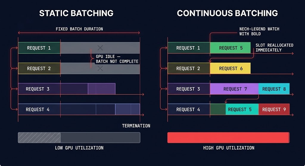
Static batching — the original inference serving model — allocates a fixed batch of requests, runs the full batch through the model until all sequences complete their generation, then processes the next batch. The problem is that sequences in a batch complete at different times. A short answer completes in 20 tokens. A long answer in the same batch takes 500 tokens. For the 480 tokens of additional generation the long answer requires, the GPU slots occupied by the short-answer sequences are idle — allocated to the batch but doing no work. GPU utilization during this tail period drops in proportion to the variance in sequence lengths across the batch. Under real production traffic, where sequence length variance is high, static batching produces GPU utilization that is structurally inefficient regardless of how much traffic is being served.
Continuous batching — also called iteration-level or dynamic batching — processes inference at the token generation level rather than the sequence level. When a sequence in the batch completes, its GPU slot is immediately reallocated to a new incoming request from the queue. The batch is not a fixed unit that runs to completion — it is a continuously refilled pool of active token generation operations. The result is consistently higher GPU utilization, lower queue depth under sustained load, and the 2–4x throughput improvement over static batching that production benchmarks consistently show. Continuous batching transformed inference serving from request-response execution into queue-optimized runtime orchestration — and that transformation changes how you instrument it, how you size it, and how it fails.
The instrumentation consequence: queue depth and slot utilization are more operationally meaningful than request count and average latency for continuous batching runtimes. A serving stack processing 1,000 requests per minute with static batching and one processing the same load with continuous batching look identical in request count metrics. They look very different in slot utilization, queue depth variance, and P99 TTFT distribution. If you are monitoring a continuous batching serving stack with request-count and average-latency metrics, you are monitoring the wrong layer.
The failure consequence: continuous batching instability under burst traffic is a different failure mode than static batching timeout. When continuous batching slots fill faster than sequences complete — under a traffic spike with high token-length requests — the queue grows, slot reallocation frequency drops, and P99 TTFT climbs. The failure looks like latency degradation, but the root cause is slot exhaustion, not hardware saturation. GPU utilization may look healthy throughout. This is the physics behind the Concurrency Collapse Without Saturation failure mode, which Section 6 covers in full.
Speculative decoding provides a complementary throughput mechanism — using a small draft model to generate candidate token sequences that a larger verification model accepts or rejects in a single parallel forward pass. For workloads where the draft model’s predictions are frequently correct (structured outputs, domain-constrained responses, predictable completion patterns), speculative decoding can reduce effective TTFT significantly without changing the model quality of verified outputs. The operational overhead is the draft model itself: additional GPU memory, a second artifact in the governance bundle, and a second version dependency in the deployment configuration.
KV cache management and session affinity are the serving layer mechanisms that govern multi-turn and RAG workload efficiency. The KV cache stores intermediate attention computations for previously processed tokens — reusing it for follow-up requests in a multi-turn session avoids recomputing the full conversation context on every turn. Session affinity — routing requests from the same session to the same serving instance — is the infrastructure prerequisite for cache reuse. Without it, every turn lands on a different instance, every turn recomputes from context, and the per-request compute cost scales with conversation depth rather than remaining bounded. At scale, for multi-turn workloads, the absence of session affinity is not a minor inefficiency — it is a structural cost multiplier that no token ceiling or routing optimization can compensate for.
Serving framework selection — vLLM, NVIDIA TensorRT-LLM, Triton Inference Server — is a decision with physics consequences that cannot be undone without a full serving stack migration. vLLM’s continuous batching and PagedAttention memory management make it the strongest general-purpose choice for high-concurrency inference with mixed request lengths. TensorRT-LLM delivers better throughput for fixed-shape workloads where the model architecture and sequence length distribution are stable and optimization for a specific GPU type is justified. Triton is the right choice for multi-framework serving environments where model heterogeneity requires a common serving abstraction across different model types and backends. The selection criterion is workload profile, not feature list — matching the serving framework’s optimization target to the actual request distribution the production system will receive.
The Concurrency Stability Problem
Concurrency stability is the defining operational challenge of inference infrastructure at production scale — and the one most poorly understood before first exposure to a production failure.
Training infrastructure optimizes for throughput saturation. The goal is to drive GPU utilization as high as possible across the full cluster for the duration of the training run. More utilization means more gradient computation per hour means lower total training cost. Underutilization is waste. The operational objective is to eliminate it.
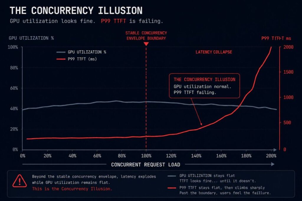
Inference infrastructure must maintain concurrency stability under unpredictable request behavior. The goal is not maximum utilization — it is predictable P99 TTFT across a continuous stream of requests that vary in length, context depth, concurrency level, and computational demand. High utilization is not intrinsically good for inference. A serving stack running at 90% GPU utilization with stable P99 TTFT is performing correctly. A serving stack running at 65% GPU utilization with degraded P99 TTFT is failing — and the failure is invisible to any monitoring that uses GPU utilization as its primary signal.
This is the Concurrency Illusion: a cluster may appear underutilized while already operating beyond its stable concurrency envelope.
The mechanics of concurrency collapse follow a consistent cascade. Variable token-length requests in a continuous batching queue create fragmented slot utilization — short sequences complete and free slots, long sequences hold slots for extended periods, and the effective throughput of the batch pool drops below its nominal capacity without any hardware metric showing degradation. KV cache fragmentation compounds this: as concurrent sessions accumulate context, the available KV cache memory becomes increasingly fragmented across session boundaries, increasing eviction frequency and forcing partial recomputation. Eviction-triggered recomputation increases per-request latency. Increased per-request latency increases slot hold time. Increased slot hold time reduces effective concurrency. P99 TTFT climbs. The cascade is self-reinforcing.
Burst traffic behavior interacts with this cascade in a particularly damaging way. A traffic spike increases queue depth. The autoscaler detects the queue buildup and launches additional serving instances. New instances start with empty KV caches — every session routed to a new instance recomputes from context. Cold-start recomputation increases the per-request compute load on the new instances precisely when they are absorbing overflow traffic. The new instances enter their own concurrency instability cascade before their KV caches warm. The autoscaler has distributed the concurrency collapse rather than resolving it.
Tail latency amplification is the observability signature of concurrency instability. P99 TTFT climbs while P50 TTFT remains stable — the average user experience looks fine while the tail experience degrades. This divergence between P50 and P99 latency is diagnostic: it indicates that a subset of requests is disproportionately delayed, which in a continuous batching context typically means long-context requests are holding slots for extended periods while shorter requests cycle through normally. The fix is not more hardware. It is serving runtime configuration: separate queue tiers for requests above and below a context-length threshold, aggressive KV cache eviction policies for sessions that have not sent a follow-up request within a defined window, and concurrency limits set at the serving layer rather than inferred from hardware utilization.
Retry storm interaction is the final amplification layer. Users or downstream systems that receive latency-degraded responses often retry. Retries add new requests to a queue that is already under pressure. Additional queue depth increases slot competition. Increased slot competition increases latency. Increased latency increases retries. The retry storm is not a separate failure mode from concurrency collapse — it is the behavioral response to a physics failure, and it is what turns a manageable latency degradation event into a full serving stack incident. The retry storm architecture maps how this behavioral amplification pattern develops in agentic systems specifically, where retry logic is embedded in agent frameworks rather than in end-user clients.
Token-length variance is the primary driver of KV cache fragmentation at the serving layer. A serving stack that receives requests with highly variable context lengths — some 100 tokens, some 8,000 tokens — cannot allocate KV cache efficiently without explicit memory management. PagedAttention, vLLM’s memory management approach, addresses this by allocating KV cache in fixed-size pages rather than contiguous blocks — allowing non-contiguous memory allocation that reduces fragmentation without requiring upfront reservation of worst-case memory per session. The operational consequence for architecture: serving frameworks that implement PagedAttention or equivalent non-contiguous KV cache management are significantly more stable under variable-length workloads than those that use contiguous per-session allocation.
Multimodal request asymmetry extends the token-length variance problem into a second dimension. Vision-language and audio-language models process input modalities with fundamentally different token counts — an image tokenizes to hundreds or thousands of tokens, an equivalent text description to dozens. Mixed multimodal and text-only request streams hitting the same serving pool create extreme token-length variance that fragments KV cache and destabilizes concurrency far beyond what text-only variable-length workloads produce. Multimodal inference workloads require explicit serving tier separation — dedicated serving pools per modality class with queue management tuned to the token-length distribution of each class.
The correct concurrency instrumentation target for production inference is not GPU utilization. It is the combination of queue depth trend, slot utilization variance, KV cache pressure, and P99 versus P50 TTFT divergence measured together as a concurrency health signal. When these four metrics are tracked simultaneously, concurrency collapse becomes detectable before it becomes a user-visible incident. When only GPU utilization is tracked, the Concurrency Illusion persists until the incident report arrives.
The Cost Governance Layer
Inference cost is a behavioral property of the runtime, not a physical property of the hardware. That distinction is not semantic — it determines what governance architecture is capable of controlling inference spend and what is structurally blind to it.
Traditional cloud cost governance was built for a world where cost followed provisioning. You allocated resources, you paid for the allocation, and you optimized by right-sizing the allocation to the actual utilization. FinOps tooling, reservation models, and cost attribution dashboards were all built on this assumption. Inference breaks it at every layer. You can provision the exact right GPU count, at the exact right tier, with the exact right reservation — and still have inference spend compound past every forecast. Because the cost driver is not the infrastructure you provisioned. It is what agents, workflows, and users do with it at runtime: how many tokens they consume per request, how often they retry, how deep the agentic execution loops run, how much retrieval context gets injected into every prompt. None of these are visible to FinOps tooling built for EC2 optimization. All of them are the actual cost signal.
The teams getting blindsided by inference spend are not making operational mistakes in the traditional sense. They are applying a cost model that was never designed for the cost structure they are operating. GPU utilization can read 70% — a healthy number by any provisioning-era standard — while inference spend doubles through behavioral drift that lives entirely above the GPU layer. The inference cost architecture maps this structural mismatch in full. The governance architecture that closes it operates at the runtime layer, not the billing layer.
The cost governance layer interaction with the traditional FinOps model for AI workloads is one of replacement, not extension. FinOps practices built for reservation optimization, commitment management, and utilization right-sizing remain valid for the infrastructure that inference runs on. They are not valid for governing what inference costs. That requires a separate instrumentation model — per-request token consumption logged with every request, retry rates tagged with agent and workflow identity, cost attributed at the workflow level — and a separate enforcement model — execution budgets, routing constraints, and loop depth limits enforced in the serving gateway rather than reported after the billing period closes.
Retrieval Changes Inference Physics
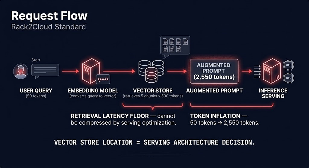
Retrieval Augmented Generation is widely treated as an application architecture pattern — a way to ground model outputs in current, domain-specific knowledge without retraining. That framing is correct at the application layer. It is incomplete at the infrastructure layer. When retrieval enters the inference path, it does not add an application step before a serving call. It changes the physics of the inference infrastructure itself — the latency floor, the token economics, the concurrency behavior, the egress costs, and the placement constraints all shift in ways that cannot be addressed by optimizing the serving layer alone.
The infrastructure consequence of retrieval is a hard latency floor that sits below the serving layer and cannot be compressed by serving optimization. A serving runtime that delivers 80ms median TTFT for direct inference calls will not deliver 80ms TTFT for RAG-augmented requests if the vector database query adds 50ms of retrieval latency. The retrieval latency is not a serving problem. It is a placement and infrastructure problem. The only architectural levers that address it are co-location (placing the vector store and inference endpoints in the same availability zone or rack), retrieval caching (pre-computing and caching retrieval results for frequent queries), and embedding index sharding (distributing the index to reduce per-query scan depth). Serving-layer optimization cannot recover latency that is consumed before the serving layer receives the fully-augmented prompt.
The Vector Databases and RAG architecture covers how retrieval systems are designed, governed, and optimized — embedding pipelines, index topology, chunking strategy, hybrid retrieval, and sovereign vector store patterns. This section ends at the boundary between infrastructure consequence and retrieval implementation: the physics of what retrieval does to inference behavior, and why those physics must inform placement and serving architecture decisions before the retrieval system is designed. The two pages are complementary — this page owns the infrastructure impact, the RAG page owns the retrieval architecture.
The Observability Layer
The observability layer for inference infrastructure must instrument two domains simultaneously that traditional monitoring was designed to cover only one of. GPU utilization, memory consumption, request throughput, and error rates are physics-layer signals — they surface hardware state and serving runtime health. They do not surface behavioral state. Token consumption per request, retry rate per agent, cost per workflow, and output characteristic drift are behavioral signals — they surface what the runtime is doing with the infrastructure, which is what determines cost and quality over time.
Most production inference deployments instrument the physics layer adequately and the behavioral layer not at all. The result is an observability architecture that can detect hardware failure and serving downtime, but cannot detect the drift patterns that produce the expensive failures: behavioral cost compounding, concurrency envelope degradation, retrieval-induced token inflation, and silent model drift that changes output characteristics without triggering any infrastructure alert.
The instrumentation decisions that enable this observability coverage must be made at architecture time — before the first production deployment, not after the first anomaly surfaces. Per-request token consumption must be logged with the request, not derived post-hoc from billing data. KV cache pressure must be exposed as a serving-layer metric by the serving framework, not inferred from latency variance. Retry rates must be tagged with agent and workflow identity at the point of retry. Output characteristic distributions must be computed over rolling windows and compared against baselines at the observability layer, not evaluated as individual outliers by a human reviewer.
The operational principle applies to both domains equally: you can only detect what you instrument for, and you can only instrument for what you decide to measure before the failure occurs. Inference systems fail through drift in the behavioral domain and through instability in the physics domain. Neither is visible to monitoring designed only for the other. The autonomous systems drift analysis maps how behavioral drift compounds in agentic inference systems specifically — the accumulation pattern that makes drift the most expensive class of inference failure and the hardest to remediate after it has been running undetected.
Inference Deployment Models
Not all inference workloads require the same deployment architecture. The deployment model determines the cost structure, the operational overhead, the latency profile, and the scaling behavior of the inference system. Defaulting to a single deployment model across all workload classes is the infrastructure equivalent of running every cloud workload on the same EC2 instance type — technically functional, economically indefensible at scale.
| Workload Type | Deployment Model | Governing Constraint | When to Reconsider |
|---|---|---|---|
| Experimental internal copilots, early-stage AI | Managed cloud inference endpoints | Iteration velocity — model selection still in flux, utilization unpredictable | Utilization stabilizes above 40% consistently; model selection hardens |
| Stable high-volume inference, predictable demand | Dedicated GPU endpoints, reserved capacity | Concurrency economics — reserved capacity delivers better price-performance than on-demand above sustained 50–60% utilization | Token volatility returns; workload profile shifts significantly; model changes frequently |
| Sovereign enterprise AI, regulated workloads | On-premises inference cluster, local control plane | Data governance — regulatory or security constraints prohibit external control plane dependency | Sovereignty requirements relax; compliance framework changes; cloud sovereign region becomes available |
| Multi-region, latency-sensitive inference | Edge or colocated inference, geographically distributed | TTFT geography — physics of network distance impose a latency floor that cannot be optimized away without proximity to the user | Latency tolerance widens; consolidation becomes viable; regional traffic volumes drop below the threshold that justifies distributed capacity |
| Agentic and multi-step workflow infrastructure | Hybrid inference topology, tiered routing across model sizes | Retry amplification and token volatility — agentic systems produce unpredictable token consumption that requires both burst capacity and cost enforcement simultaneously | Agentic behavior stabilizes and hardens; token consumption becomes predictable; dedicated tier becomes justified |
| Retrieval-heavy enterprise RAG | Co-located inference and vector layer, shared placement | Retrieval latency and egress gravity — the retrieval latency floor and cross-zone egress costs impose placement constraints that serving optimization cannot address | Vector index migrates; co-location advantage shifts; retrieval latency floor drops below serving-layer latency through infrastructure improvement |
| Burst inference workloads, variable demand | Cloud burst capacity above a reserved on-prem or dedicated baseline | Capacity volatility — burst demand cannot be served cost-effectively by owned infrastructure sized for peak; baseline demand cannot be served cost-effectively by on-demand cloud | Burst patterns harden into predictable demand; reserved capacity covers the full range; burst frequency drops below the threshold that justifies hybrid complexity |
The reassessment trigger column is the most operationally important column in this table. Inference deployment decisions decay — the conditions that made a deployment model correct at month one change as utilization stabilizes, workload behavior hardens, model selection settles, and the economics of ownership versus rental shift. Treating the initial deployment model as permanent is how organizations end up with inference infrastructure that was correctly designed for their situation eighteen months ago and is structurally mismatched to their current scale and cost profile. Inference placement is dynamic architecture, not a one-time deployment decision.
The Inference Placement Economics Decision
Inference workloads have a property that training workloads do not: they stabilize. Training runs are bounded events — they start, they finish, the cost event closes. Inference is continuous, and continuous workloads develop predictable patterns over time. Request volume stabilizes. Token consumption per request stabilizes. Concurrency profiles harden. The workload becomes, in the language of infrastructure economics, a steady-state system — and steady-state systems have fundamentally different placement economics than experimental or bursty systems.
This stabilization is what makes inference placement economics a decision that must be revisited as workloads mature, not a decision made once at deployment. The cloud-first default that is correct for experimental AI becomes economically indefensible for stable, high-volume inference. The on-prem investment that is unjustifiable for unpredictable early-stage workloads becomes the correct economic choice when utilization hardens above the break-even threshold. The placement decision is not cloud versus on-prem. It is a multi-variable economics calculation that changes as the workload changes.
The eight variables that govern the inference placement economics decision:
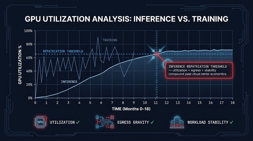
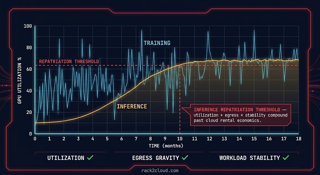
The repatriation calculus for inference workloads differs from the general cloud repatriation argument in one important structural way: inference is the first AI workload class to justify repatriation because it is the first to stabilize. Training workloads remain unpredictable in demand, bursty in utilization, and experimental in model selection — the properties that make cloud economics favorable persist throughout the training lifecycle. Inference workloads, once a model is in production and serving real traffic, begin hardening immediately. The utilization pattern stabilizes within weeks. The token economics stabilize within months. The concurrency profile becomes predictable. The economics of repatriation follow the stabilization curve — and for organizations running high-volume inference at cloud GPU rates, the repatriation calculation becomes favorable earlier than most infrastructure planning cycles anticipate.
Decision Framework
Every inference architecture decision has a right answer for the scenario it is solving. The framework below maps the placement decision — not the serving stack selection, which is covered in the Serving Layer section — to the governing constraint and the signal that should trigger a reassessment.
| Inference Scenario | Placement Model | Governing Constraint | Reassessment Trigger |
|---|---|---|---|
| Early-stage AI, model selection in flux | Cloud-first, managed endpoints | Iteration velocity — capital commitment before model stability is waste | Consistent utilization above 40%; model selection hardens for 90+ days |
| Production inference, stable demand above 60% utilization | Reserved dedicated capacity or on-prem migration | Utilization economics — cloud GPU rate exceeds owned amortization at this utilization level | Utilization drops below 50% for 60+ days; model churn increases; workload profile shifts |
| Regulated AI, data sovereignty required | On-premises inference cluster, sovereign control plane | Non-economic — regulatory compliance is the constraint regardless of utilization | Regulatory framework changes; sovereign cloud region becomes compliant option |
| Interactive global AI, sub-100ms TTFT required | Geographically distributed edge inference | Latency geography — network physics impose a floor that centralized infrastructure cannot serve below | Latency requirement relaxes; user geography consolidates; network infrastructure improves regional latency |
| RAG-heavy enterprise application | Co-located inference and vector store | Retrieval latency floor and egress gravity — placement of index determines TTFT floor and egress cost | Vector index migrates; retrieval frequency drops; embedding gravity shifts |
| Agentic multi-step workflows | Hybrid topology, dedicated baseline with burst capacity | Token volatility — agentic systems produce unpredictable peak token demand that owned baseline cannot absorb economically | Agent behavior stabilizes; token consumption hardens into a predictable range; burst headroom shrinks |
| High-volume inference approaching repatriation threshold | On-prem migration from cloud reserved | Inference Repatriation Threshold — utilization + egress gravity + workload stability compound past the economics of cloud rental | Annual review of utilization trend, egress cost model, and silicon amortization schedule |
You’ve seen how inference infrastructure is architected across silicon, serving, concurrency, cost governance, and placement economics. The pages below cover the layers it runs on, the systems that feed it, and the governance discipline that makes it operationally controllable.
Architect’s Verdict
Inference is where AI infrastructure cost is actually produced and where AI infrastructure failures are actually felt. Training is bounded and visible — the bill is large, arrives once, and can be planned for. Inference is continuous, behavioral, and compounding — it accumulates through token consumption, retry amplification, agentic loop depth, and retrieval inflation in ways that standard infrastructure monitoring was never designed to surface.
The organizations building AI infrastructure correctly are not the ones with the most capable models or the most sophisticated serving stacks. They are the ones who modeled both governing domains — physics and behavior — before the first production deployment, designed their concurrency envelope before discovering it under load, built cost governance into the runtime before behavioral spend compounded past forecast, and planned their placement economics as a dynamic decision that would require reassessment as workloads stabilized.
- [+]Model inference cost as a behavioral property — token consumption, retry frequency, agentic depth — not a provisioning property
- [+]Design the concurrency envelope before production deployment — locate the stability boundary in staging, not in an incident report
- [+]Instrument both physics signals (TTFT P99, KV cache pressure, queue depth) and behavioral signals (token trend, retry rate per agent, cost per workflow) before the first production deployment
- [+]Co-locate inference endpoints with retrieval infrastructure — the vector index location is a serving architecture decision, not an application design detail
- [+]Revisit placement economics as workloads stabilize — the deployment model correct at month one is frequently wrong at month twelve
- [+]Separate training and inference silicon — the hardware optimization targets are different; running both on shared infrastructure conflates two problems that require separate solutions
- [!]Use GPU utilization as a proxy for inference health — a cluster at 65% utilization can be failing concurrency stability while a cluster at 85% can be operating correctly
- [!]Set TTFT targets without modeling the retrieval latency floor — serving optimization cannot compress latency that is consumed before the serving layer receives the prompt
- [!]Deploy agentic inference workloads without loop depth limits and token budgets enforced in the runtime — behavioral cost amplification is invisible until the billing cycle surfaces it
- [!]Treat the initial placement decision as permanent — inference workloads stabilize, and the economics that justified cloud-first at month one shift as utilization hardens
- [!]Rely on autoscaling to resolve concurrency collapse — new instances start cold, and cold-path storms under the load that triggered scaling can worsen the latency event they were meant to relieve
- [!]Provision inference silicon before modeling egress gravity — cross-zone retrieval costs and embedding locality constraints may make the cheapest GPU option the most expensive total infrastructure choice
The AI Architecture Learning Path provides the sequenced reading order for architects building the complete stack — from silicon and fabric through inference architecture, LLM operations governance, and the retrieval layer that changes inference physics when RAG enters the design.
You’ve Mapped the Inference Layer.
Now Find Out Where Yours Has Gaps.
Inference infrastructure failures — concurrency collapse, behavioral cost compounding, retrieval-induced latency floors, and placement misalignment — are architecture problems that compound quietly before they become expensive. The triage session identifies which gaps exist in your stack before a production incident or a quarterly billing surprise makes them visible.
AI Infrastructure Audit
Vendor-agnostic review of your inference architecture — silicon placement and hardware split, serving runtime configuration and concurrency envelope, cost governance and execution budget coverage, retrieval co-location and egress modeling, and placement economics relative to current utilization and workload stability.
- > Silicon placement and hardware split validation
- > Serving runtime and concurrency envelope review
- > Cost governance and execution budget audit
- > Placement economics and repatriation threshold assessment
Architecture Playbooks. Every Week.
Field-tested blueprints from real inference infrastructure environments — concurrency collapse post-mortems, behavioral cost runaway analysis, retrieval latency floor case studies, and the placement economics patterns that determine when inference repatriation closes.
- > Inference Concurrency & Serving Architecture Patterns
- > Behavioral Cost Architecture & Execution Budgets
- > Inference Placement Economics & Repatriation Analysis
- > Real Failure-Mode Case Studies
Zero spam. Unsubscribe anytime.
Frequently Asked Questions
Q1: What is AI inference architecture and why does it require its own discipline?
A: AI inference architecture is the discipline of designing the infrastructure that governs production AI serving — silicon selection, serving runtime configuration, concurrency stability, cost governance, and placement economics. It requires its own discipline because inference economics are governed simultaneously by infrastructure physics (latency, memory, fabric, concurrency) and runtime behavior (token consumption, retries, agentic depth, retrieval amplification). Traditional infrastructure practice was almost entirely a physics discipline. Inference requires governing both layers at once, with different instrumentation, different governance architecture, and different failure modes than any adjacent infrastructure category.
Q2: What is the Concurrency Illusion and why does it matter for inference operations?
A: The Concurrency Illusion is the condition where a serving cluster appears underutilized by GPU utilization metrics while already operating beyond its stable concurrency envelope — the range of concurrent request load within which the serving runtime maintains acceptable P99 TTFT. GPU utilization measures compute density, not concurrency stability. A cluster at 65% GPU utilization can be in active concurrency collapse — with P99 TTFT climbing, queue depth growing, and KV cache fragmenting — while standard monitoring shows nothing anomalous. The Concurrency Illusion explains why inference systems fail “early,” why autoscaling frequently worsens latency rather than relieving it, and why GPU utilization is the wrong primary signal for inference health.
Q3: How does retrieval change inference infrastructure requirements?
A: Retrieval introduces a hard latency floor below the serving layer that cannot be addressed by serving optimization alone. Every RAG request carries minimum latency equal to the retrieval query time plus the network round-trip to the vector store — and no serving framework optimization can recover latency consumed before the augmented prompt arrives at the serving layer. Retrieval also introduces token inflation (retrieved chunks increase prompt length, increasing KV cache pressure and per-request compute), egress costs that compound at inference frequency, and request fan-out that disrupts continuous batching queue management. The architectural implication: the location of the vector index is a serving architecture decision, not an application design detail.
Q4: When does inference repatriation become economically justified?
A: The Inference Repatriation Threshold is a compound indicator, not a single metric. It requires consistent GPU utilization above 60–70% for 90+ days, retrieval egress costs that are material relative to compute costs, token economics that have stabilized within a predictable range, and a concurrency profile that can be right-sized to dedicated hardware without significant overprovisioning. When all four are present simultaneously, the economics of on-premises inference typically close within 12–18 months of hardware acquisition cost. Inference is uniquely suited to repatriation among AI workload classes because it stabilizes over time — training remains bursty and experimental, inference hardens into predictable steady-state patterns that owned infrastructure can be right-sized for.
Q5: Why is continuous batching the defining architectural shift in inference serving?
A: Static batching allocates a fixed request batch and runs it to completion before processing new requests — GPU slots held by completed short sequences idle while long sequences in the same batch finish. Continuous batching processes at the token generation level: when any sequence completes, its slot is immediately reallocated to a new request from the queue. The result is 2–4x throughput improvement over static batching at equivalent hardware cost, consistently higher GPU utilization, and lower queue depth under sustained load. More importantly, it transforms serving from request-response execution into queue-optimized runtime orchestration — which changes the failure modes, the instrumentation targets, and the sizing methodology for the entire serving layer.
Q6: How should inference cost governance be architected differently from traditional cloud FinOps?
A: Traditional FinOps governs provisioning-based cost — allocate resources, measure utilization, optimize through right-sizing and reservation. Inference cost is behavioral — it accumulates through token consumption rates, retry frequency, agentic loop depth, and retrieval amplification, none of which are visible to provisioning-based monitoring. The governance architecture that controls inference cost operates at the runtime layer: token ceilings and execution budgets enforced at the inference gateway before tokens are generated, tiered model routing that matches request complexity to model capability, and workflow-level cost attribution that tracks cost per request per workflow over time. FinOps tooling built for EC2 optimization can govern the infrastructure inference runs on. It cannot govern what inference costs — that requires a separate instrumentation model at the behavioral layer.
Q7: How does the AI Inference Architecture page relate to the other AI infrastructure sub-pages?
A: The AI Infra pillar has clean ownership boundaries by design. GPU Orchestration governs silicon scheduling and CUDA isolation — the accelerator layer below inference serving. Distributed AI Fabrics governs the network backplane that determines P99 latency for sharded inference and distributed model deployment. AI Inference Architecture governs runtime infrastructure and placement economics — silicon selection, serving design, concurrency stability, cost governance, and where inference workloads belong as they scale. LLM Operations Architecture governs the operational control plane above the infrastructure — artifact management, lifecycle, rollback, and runtime authority governance. Vector Databases and RAG governs the retrieval layer whose placement changes inference physics. Each page owns a distinct layer. This page is the infrastructure and economics layer.