PERFORMANCE MODELING PATH
PREDICTING FAILURE BEFORE IT HAPPENS.
Why Performance Modeling Matters
Most infrastructure teams measure performance. Very few model it.
Monitoring tells you what happened. Dashboards tell you what is happening. Performance modeling tells you what will happen when the system is stressed.
That difference is architectural. Modern infrastructure is not a collection of independent systems. It is a tightly coupled execution model where:
- CPU scheduling interacts with storage replication
- Storage amplification interacts with network buffers
- Network congestion amplifies tail latency
- Tail latency destroys synchronous systems
Clusters rarely fail in steady-state. They fail during rebuild storms, node loss (N+1 scenarios), cross-zone traffic bursts, AI all-reduce congestion, and live migration overlaps.
Performance modeling forces you to ask the real question: What does this cluster look like under duress?
This Learning Path teaches you to model resource contention, latency envelopes, and failure amplification before production exposes them. No vendor sizing calculators. No “it should be fine.” Only deterministic math.
The System Model: Performance Is an Equation
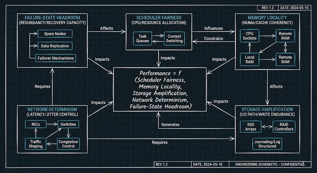
Performance is not a metric. It is a function. In modern infrastructure:
Performance = f (Scheduler Fairness, Memory Locality, Storage Amplification, Network Determinism, Failure-State Headroom)
These variables are not independent.
- Increase replication factor and you increase CPU overhead.
- Increase CPU contention and you amplify tail latency.
- Increase network congestion and synchronous systems stall.
- Reduce headroom and every failure becomes nonlinear.
This Learning Path treats infrastructure as a coupled system, not isolated components. We are not modeling parts. We are modeling interaction surfaces.
Who Should Read This
If you are responsible for predicting infrastructure behavior—not just reacting to it—this is for you.
- Virtualization Engineers: You need to understand CPU Ready vs CPU Wait, NUMA exposure, and scheduler saturation before clusters degrade silently.
- Storage Architects: You must quantify write amplification, rebuild traffic, and RF2/RF3 physics under load.
- Network Engineers: You care about microbursts, incast collapse, ECN behavior, and P50 vs P99 latency divergence.
- AI / HPC Infrastructure Teams: You operate synchronous GPU clusters where one delayed node defines global performance.
- Platform & Cloud Architects: You size for N+1 and N+2—not marketing steady-state.
(If you are new to virtualization physics, begin with the Modern Virtualization Architecture Pillar to establish scheduler and NUMA control-plane fundamentals.)
The Core Modeling Dimensions
Performance modeling is not about a single metric. It is about interaction surfaces.
Phase 1: CPU Scheduling Physics
Clusters do not run out of CPU. They run out of scheduling fairness.
Key modeling variables:
- vCPU:pCPU ratio
- NUMA alignment
- CPU Ready (%RDY)
- CPU Wait (distributed storage contention)
- Interrupt pressure
- Steal time in virtualized cloud
Deep Dive: Resource Pooling Physics: CPU Wait & Memory Ballooning
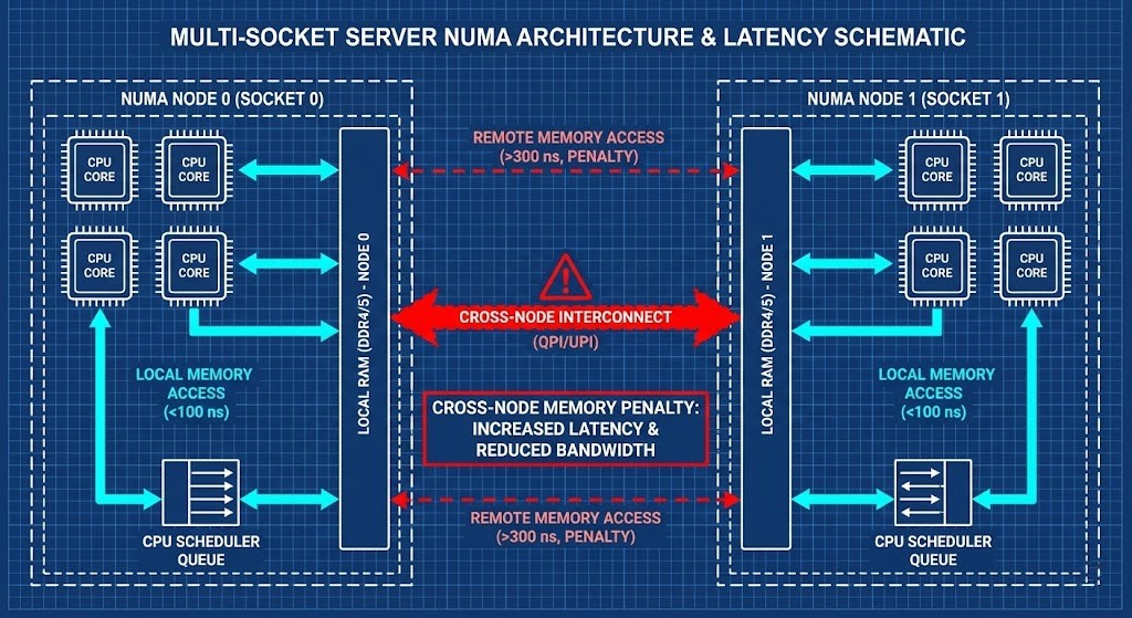
Phase 2: Memory & NUMA Topology
Memory modeling is not capacity modeling. It is:
- Remote memory %
- NUMA rebinding after migration
- Ballooning thresholds
- Page cache interference
- AI model memory residency
A 4 vCPU VM behaves differently when rebinding across NUMA domains. Memory locality is performance.
Phase 3: Storage Convergence Modeling
In HCI systems, storage is not “behind” compute. It is inside it. You must model:
- Write amplification (RF2 vs RF3)
- Controller VM overhead (CVM tax)
- Rebuild bandwidth
- Metadata amplification
- Checkpoint overlap (AI training workloads)
Rebuild modeling example: If a node fails, replication traffic increases, CPU overhead increases, network east-west traffic increases, and your latency envelope shifts.
Deep Dive: Performance Modeling the VMware Evacuation: Nutanix AHV vs Proxmox Ceph
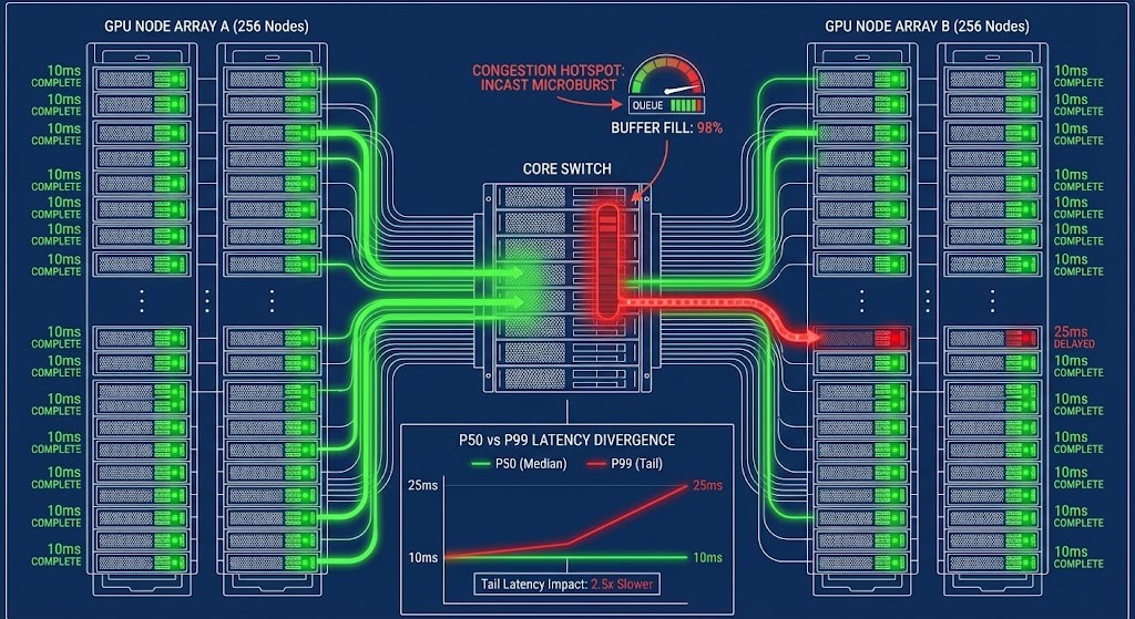
Phase 4: Network Determinism & Tail Latency
Raw bandwidth does not equal predictability. You must model:
- Microburst behavior
- Switch buffer limits
- ECN vs PFC interactions
- Incast amplification
- Cross-rack congestion
- P50 vs P99 latency divergence
In synchronous systems (e.g., AllReduce), one delayed node defines cluster time. Example: 511 nodes complete in 10ms. 1 node completes in 25ms. Global job latency = 25ms. That is tail amplification.
Phase 5: Failure-State Amplification (N+1 Modeling)
If your model only works at steady-state, it is useless. You must validate:
- Node failure + active rebuild
- ToR failure + migration overlap
- Cross-zone replication lag
- Mixed workload contention
- AI + legacy VM coexistence
Deterministic architects model the % latency increase under node loss, % CPU overhead increase, storage I/O during rebuild, and network headroom during burst.
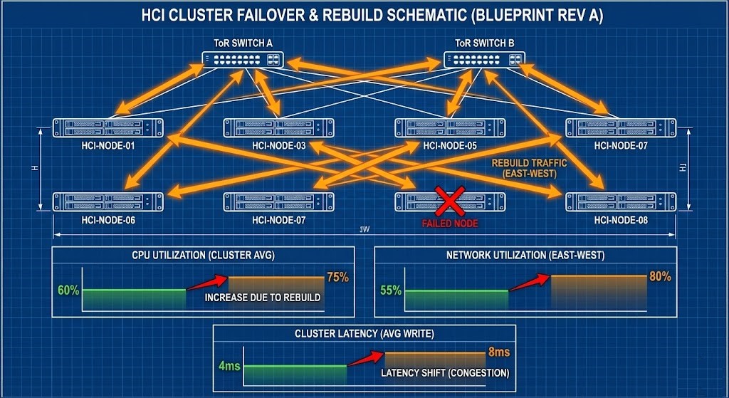
Failure-State Example: 8-Node HCI Cluster Under Duress
Consider an 8-node HCI cluster running at a steady-state CPU utilization of 60%, network utilization of 55%, with RF2 replication and a P99 storage latency of 4ms.
One node fails. Rebuild traffic consumes:
- +15% CPU across surviving nodes
- +25% east-west network bandwidth
- Increased metadata operations per write
New state:
- CPU rises to 75%
- Network rises to 80%
- P99 latency doubles to 8ms
Applications still function—but tail latency has shifted. If a second stressor overlaps (live migration, AI checkpoint burst, or cross-zone replication), the cluster enters the collapse envelope. This is why modeling cannot stop at averages.
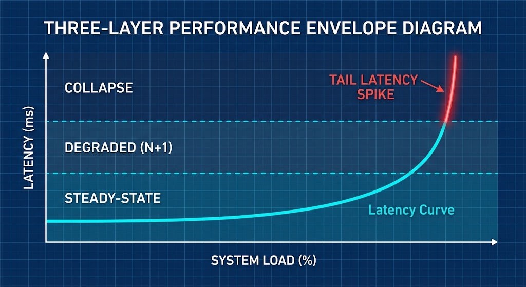
The Envelope Model: Steady, Degraded, Collapse
Every engineered cluster operates inside three envelopes:
- Steady-State Envelope: Normal operating conditions with predictable P50 and bounded P99.
- Degraded Envelope (N+1): One fault domain lost. Rebuild traffic active. Latency increases but SLOs hold.
- Collapse Envelope: Headroom exhausted. Tail latency spikes. Synchronous workloads stall.
Most teams only measure steady-state. Deterministic architects validate the degraded envelope. If your SLO survives steady-state but fails at N+1, the cluster was never production-ready.
Modeling Methodology
Performance modeling is not guesswork. Use this structured approach:
Step 1: Define the Baseline Envelope
- Steady-state CPU utilization, Storage P50/P99 latency, Network headroom %, Memory locality %.
Step 2: Inject Controlled Stress
- Simulate node loss, active rebuilds, burst traffic, migration events, or AI checkpoint spikes.
Step 3: Measure Envelope Shift
- Track P99 latency increase, CPU Ready delta, storage amplification %, network buffer pressure, and application error rates.
Step 4: Validate Against SLO
- If SLO breaks under N+1: Cluster is under-sized.
- If SLO breaks only at N+2: Cluster may be correctly engineered.
Observability: Modeling Defines the Envelope, Telemetry Verifies Drift
Modeling predicts behavior under stress. Observability confirms whether the system remains inside its validated envelope.
- Monitoring answers: What happened?
- Telemetry answers: Where is saturation forming?
- Modeling answers: When will it fail?
Without modeling, dashboards are forensic. Without observability, models are theory. Deterministic infrastructure requires both.
Deterministic Tools Integration
This Learning Path integrates directly with the Rack2Cloud Deterministic Tools Inventory. Stop guessing and start calculating:
- Metro Latency Scout: Validate RTT thresholds and network determinism for synchronous storage and stretch-cluster stability.
- AI Ceph Throughput Calculator: Estimate aggregate bandwidth, Ceph node counts, and Erasure Coding overhead for distributed AI training clusters.
- VMware Core Calculator: Benchmark core-to-license ratios to accurately model your compute and NUMA footprint for Broadcom VVF/VCF environments.
- Cloud Egress Calculator: Model the true data movement physics and transfer times when routing workloads out of the public cloud.
Model first. Then deploy.
Performance Collapse Has Economic Physics
Performance modeling is also cost modeling.
Under-sizing results in: GPU idle burn in AI clusters, SLA penalties, operational fire drills, and emergency hardware procurement. Over-sizing results in: Idle silicon, licensing waste, and excess power and cooling spend.
The goal is not maximum headroom. The goal is deterministic headroom. Performance modeling allows architects to size for N+1 with precision—not fear.
Common Performance Modeling Myths
| Myth | The Deterministic Reality |
| “Average utilization is fine.” | Tail latency determines system health. |
| “10GbE is enough for Ceph.” | Depends on replication factor, rebuild concurrency, and AI checkpoint overlap. |
| “More nodes = linear scale.” | Scheduler fairness, metadata overhead, and network incast define scaling limits. |
| “We’ll monitor it after go-live.” | Monitoring is forensic. Modeling is preventative. |
Continue the Architecture Journey
Performance modeling is the connective tissue between your primary infrastructure pillars. Expand your matrix:
- Modern Virtualization Learning Path
- Modern Compute Learning Path
- Storage Architecture Learning Path
- Networking Architecture Learning Path
- HCI Architecture Learning Path
- Migration Strategy Learning Path
Q: Is performance modeling just capacity planning?
A: No. Capacity planning is static. Modeling simulates dynamic failure states and contention physics.
Q: Why does P99 latency matter more than average latency?
A: Because synchronous systems wait for the slowest participant.
Q: Should I size for steady-state or N+1?
A: N+1 minimum. N+2 for regulated or AI workloads.
Q: Is this only for HCI?
A: No. This physics applies to traditional SAN, public cloud instances, Kubernetes clusters, and AI fabrics.
Canonical Engineering References
For architects who want primary-source technical documentation beyond vendor marketing:
- VMware Performance Best Practices Guide (CPU Ready, NUMA scheduling, memory overcommit behavior)
- Nutanix AHV Performance and Best Practices (CVM overhead modeling, RF2/RF3 replication impact)
- Ceph Architecture & Performance Tuning Guide (Write amplification, recovery/backfill modeling)
- NVIDIA NCCL Performance Guide (AllReduce synchronization and tail latency physics)
- Arista Validated Designs for AI Networking (Buffer tuning, ECN/PFC modeling, leaf-spine determinism)
- Google SRE Workbook – Capacity Planning & Load Shedding (Envelope modeling and failure-state planning)
DETERMINISTIC PERFORMANCE MODELING
Performance is not about steady-state averages. Stop guessing at your P99 tail latency, CPU scheduling overhead, and distributed storage write amplification. Run your cluster physics through our deterministic calculators before you sign the hardware PO.
LAUNCH THE ENGINEERING WORKBENCH