

Patch Consumption Capacity: Deadlines Attach to Assets. Delivery Runs on Updates.
Patch consumption capacity is the rate at which a team can turn remediation obligations into completed work inside the deadlines attached to them, and a vulnerability count measures neither the workload nor the capacity to complete it. Microsoft’s November release notes list 1,094 CVEs. That figure tells a planner how much was disclosed. It does not say how many assets carry an obligation, how many distinct updates deliver the fixes, or how many assets an organization can hold in assessment, test and deployment at the same moment. BOD 26-04 makes the gap concrete, because it attaches timelines to vulnerabilities according to the state of the asset each one sits on. It does not attach a deadline to a CVE list.
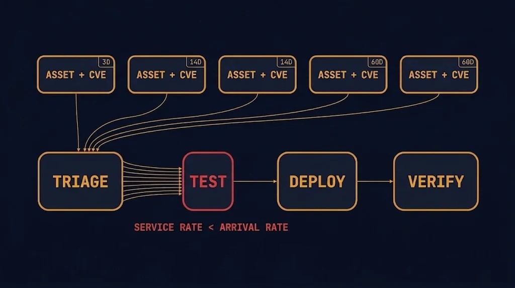
The Measurement Problem: CVE Counts Describe Vulnerabilities, Not Work
A CVE is a record of a flaw. Remediation work happens on assets, through packages, inside a pipeline that has a finite number of places to put an asset at any one time. Three different units sit behind the single number that gets quoted after every Patch Tuesday, and a plan built on the quoted number inherits the confusion. For modern infrastructure architecture, the working question for patch consumption capacity is whether the work fits inside the deadlines, and the CVE count does not answer it in either direction.
November shows why. The release notes publish a product-family table. A planner estimating patch consumption capacity from it has to separate what Microsoft states from what has to be counted independently.
| Label | Finding | Basis |
|---|---|---|
| STATED | 1,094 Microsoft CVEs in the November release. By family: Windows 726, Office 174, SQL Server 59, Developer Tools 53, SharePoint 27, Other 25, Azure 20, Exchange 9, Defender 1. The table lists distinct updates for Office (7), SQL Server (13), Developer Tools (28), SharePoint (3), Exchange (1) and Defender (1). | MSRC November 2026 release notes |
| DERIVED | In the CVRF feed, the vendor-fix remediations on Windows-named products resolve to 36 distinct KB numbers, with CVE references per KB ranging from 1 to 627. | This analysis. Method: remediations of type vendor fix, filtered to Windows-named products. The filter also catches some extension packages, and it yields 743 Windows-named CVEs against MSRC’s 726. The difference is not reconciled. |
| NOT STATED | The distinct-update count for Windows, Azure and Other (blank in the table). The number of Windows versions or builds. The November status of the lower-count KBs, which look like earlier-month packages. A definitive November Windows package total. | Not published in the release notes. Not inferred here. |
The derived row is a mapping, not an inventory. It is useful for one reason: it shows that the unit of delivery and the unit of disclosure are unrelated. By the derived mapping, at least one cumulative KB references more than 500 CVEs, so 726 Windows CVEs do not mean 726 deployments. In the other direction, one CVE on 4,000 affected, in-scope endpoints creates 4,000 asset-specific obligations, not necessarily 4,000 separate deployments. The CVE count understates the obligation count in one case and overstates the deployment count in the other.
Which obligations to work first is a separate problem. Patch visibility debt covers how confirmation lag distorts that ordering, and this post takes the ordering as given. The question here is whether the work, in any order, fits.
Three Dimensions of Patch Consumption Capacity
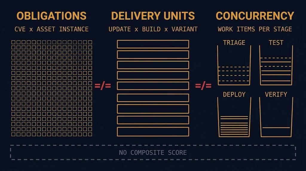
Patch consumption capacity is not one number. It has three inputs that are counted in different units and constrained by different things. The patch consumption capacity model below is a proposal, Rack2Cloud’s own, and it deliberately does not collapse into a composite score.
Obligations
An obligation is a CVE paired with an affected asset instance: what must be remediated, on which asset, by when. The asset instance carries the applicable deadline for each unresolved obligation. One asset can hold several obligations, and they can run on different clocks, because the clock depends on the state of the asset and on the attributes of the vulnerability. A CVE that affects 400 in-scope asset instances creates 400 asset-specific obligations. The count of unresolved obligations, each with its remaining time, is the demand side of patch consumption capacity.
Delivery Identity and Deployment Sequencing
Delivery identity is the update, the OS branch or build, and the architecture or package variant. It identifies what an engineer has to obtain, validate and install. One package can retire many obligations. One obligation can need different packages on different builds.
Deployment sequencing is a different thing: rings, maintenance windows, approval paths and rollout policy. A ring is an organizational choice about the order in which delivery units reach assets. It is not a property of the package. Keeping the two apart does two things. It lets the model apply to organizations that do not run rings, which still have sequencing. And it shows when sequencing, not packaging, is what limits the work. For one provider’s managed compute, managed compute patching measures the interval between the provider shipping a fix and a workload receiving it. That interval sits upstream of the delivery units counted here.
Operational Concurrency
Operational concurrency is the supply side of patch consumption capacity: the number of defined work items that each stage can hold at once. The work-item definition may differ by stage, for example an asset in triage or an asset-and-package pairing in test and deployment, but those differences must be explicit. A triage slot cannot absorb a deployment, and a deployment slot cannot absorb triage. When stage capacity is compared across different units, the work has to be converted to a common flow basis. Concurrency is also not throughput. Forty slots with a two-day cycle and forty slots with a six-day cycle are the same concurrency and very different service rates. Within each stage, concurrency and throughput have to be measured in that stage’s own work-item unit.
DIAGNOSTIC QUESTION
“If one obligation on one asset drops to a three-day clock tomorrow, which stage runs out of slots first, and who owns the path that gets it through?”
Collapsing the three dimensions into one capacity score hides which of them binds. A team with ample deployment concurrency and a two-person triage function has a triage constraint, and no average of the three will say so.
The Capacity Relationship: Little’s Law as a Planning Baseline
Little’s Law relates three averages for one defined flow: the number of work items in a system equals the rate at which they complete multiplied by the average time each spends in the system. L = λW holds only when all three variables describe the same work items and the same pipeline boundary. That is why the three dimensions have to be converted before the law is applied, and not substituted for one another.
The conversion has three steps. First, count the unresolved obligations, each with its remaining time. Second, map them to the delivery work they require on the affected assets. One deployment on one asset can retire every covered obligation on that asset, so the number of work items is not the number of obligations. Third, fix a work-item definition within each stage, and measure concurrency and throughput in that unit.
The arithmetic, using hypothetical figures that are not measured from any organization: 600 obligations map to 300 asset-and-package work items, assuming each deployment retires an average of two covered obligations. Completing those 300 work items within 14 days requires an average of about 21.4 completions per day. If that rate is sustained in a stable flow, and each work item spends an average of five days in the pipeline, including waiting, Little’s Law gives an average of about 107 work items in process. That is a flow baseline, not proof that a 300-item burst can be completed inside the deadline. The 600 obligations, the 300 work items and the 107 average work items in process are three different counts. Substituting one for another is how a plan looks feasible on paper and fails in the pipeline.
Where the Baseline Stops Being Predictive
The relationship describes averages in a stable system. A patch cycle is neither. Arrivals come in bursts: a monthly release drops hundreds of obligations at once, and out-of-band additions to the KEV catalog arrive on no schedule. Priority queues move short-clock work ahead of long-clock work and lengthen the time everything else spends waiting. Cycle times vary by platform, by owner and by the failure rate of a given package. Stages depend on each other, so a slow upstream stage starves everything behind it. And the average hides the remaining time on each asset: an obligation that has used ten of its fourteen days is a different problem from a fresh one with the same age in the average.
The baseline can show that a plan is implausible. It cannot show that a plan will meet a deadline. It is a planning check, and it is not a guarantee.
Failure Modes
Each of these is a way for the three dimensions of patch consumption capacity to disagree with each other. The order matters, because the first one is the governing rule and the following cases show how delivery policy ends up violating it.
The Earliest Unresolved Obligation Governs
The clock attaches to the unresolved obligation on a specific asset. It does not attach to the update, to the CVE or to the release. The deadline an asset is working against is the earliest remaining clock among its unresolved obligations. A queue ordered by anything else, such as package, release date or ring, can serve an obligation late, and it can do so without any single step having been wrong.
One Update, Several Obligations
A single package can satisfy several obligations on an asset, and that is the efficiency. It does so only where the package’s coverage includes each obligation. One deployment on an asset can retire every covered obligation on that asset, and a cumulative update retires the obligations whose CVEs it contains and no others. The consequence runs both ways. One short-clock obligation can pull an entire package forward for the asset it sits on, and the other obligations that package covers ride along. The same CVE can also carry different timelines on different assets, because BOD 26-04 sets timelines from four variables: asset exposure, KEV status, exploit automation and technical impact. The package is identical. The deadlines are not.
A Uniform Rollout Sequence Can Consume the Shortest Window
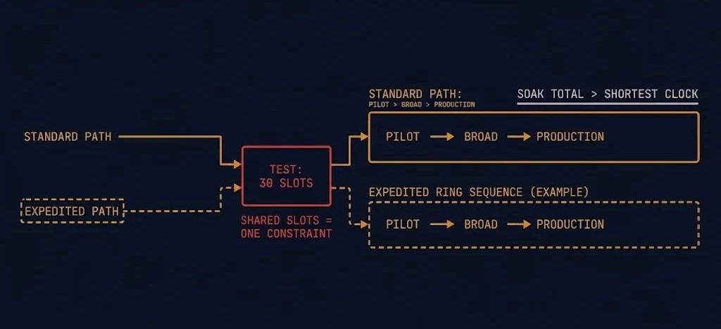
A ring sequence that runs a pilot group, then a broad group, then production, with a soak period between them, is a sound default for most obligations. If its soak periods add up to more than the shortest applicable clock, then by construction it cannot serve that clock. Applying the same sequence to every obligation is how a team ends up with a rollout policy that is correct for the 60-day work and structurally late for the 3-day work.
The architectural consequence is an expedited path: defined in advance, approved in advance, and given its own capacity. The last part is where plans usually fail. If the expedited path draws on the same triage, test and deployment slots as the standard path, then the first week with several short-clock obligations turns it into an unannounced exception to the standard path, and the shared slots are the constraint. Patch consumption capacity has to be counted per stage and per path.
The same hypothetical figures show how this looks. The flow needs about 21.4 work items a day through every stage that all items pass through. A test stage whose work item is the same asset-and-package pairing, with 30 slots and a two-day average service time, has a theoretical steady-state capacity of about 15 completions a day, before accounting for downtime, rework or other constraints. Stage capacities do not add: forty deployment slots do not offset a thirty-slot test stage, because the slots are not interchangeable. Deployment capacity can be ample and the plan still misses, because the binding stage is upstream of it. BOD 26-04’s implementation guidance places this on agency authorizing officials: they are to establish change management and continuity plans that make the timelines achievable.
Triage Is a Serial Gate
The directive’s most severe combination carries a three-day timeline plus forensic triage. The guidance says to collect evidence before patching, because patching can jeopardize artifacts, and to coordinate containment with evidence collection and patching. The timelines for the triage steps themselves are recommended, not required. Triage therefore sits in front of delivery for the highest-priority work, and it is staffed by a smaller and different group than deployment. NetScaler compromise response works through the interruption sequence for a compromised gateway appliance, evidence before update included. The capacity point here is narrower: a gate with serial service and a small number of slots caps the rate at which the most urgent work can move, whatever the deployment side can absorb.
Heterogeneous Pipelines
A fleet blends pipelines with different cycle times and different failure profiles: automated pipelines on some platforms, manual testing and manual installation on others. Planning against a fleet average hides the slow pipeline, and the slow pipeline is usually where the mission-critical systems are. The directive’s implementation FAQ gives an example of the choice this forces: prioritize staff time on manual testing and patching for mission-critical systems, and automate the rest. It also describes the timelines as maximums. Patch consumption capacity has to be planned per pipeline.
Exposure Reduction as One Potential Capacity Lever
BOD 26-04 treats mitigation as remediation, and removing a system from the internet changes its Publicly Exposed value, which shifts the timeline. Reducing exposure can therefore reduce demand on the scarce stages, subject to the directive’s own criteria. The Publicly Exposed value changes only when those criteria are actually met, so the lever exists only for assets that meet them. It is a lever with a cost. It is a change to the asset, it needs an owner and an approval path, and it consumes network and change capacity of its own. One lever among several, and not a substitute for counting.
Worked Example: BOD 26-04
CISA issued BOD 26-04 on June 10, 2026, and it revokes BOD 19-02 and BOD 22-01. Its timelines come from four variables per vulnerability: whether the asset is publicly exposed, whether the vulnerability is in the KEV catalog, whether exploitation is automatable, and the technical impact. The directive is phased. In the first phase, agencies monitor KEV and remediate according to the applicable KEV timelines. A later phase brings in the broader Table 1 timelines for every vulnerability, and that phase is dated to December 7, 2026, which is 180 days from issuance. FedRAMP’s notice uses the same date. December 7 is when the broader obligation set is scheduled to be in force. It is not the date vulnerability work begins, and it does not mean every agency is already meeting the full regime.
The directive’s mechanics matter to the patch consumption capacity model. Days are calendar days. The clock starts at the earlier of the KEV addition or the agency’s identification of the vulnerability through CDM. Mitigation counts as remediation. The timelines range from three days, with forensic triage at the most severe combination, through 14 and 60 days, to fixing the vulnerability on system upgrade at the far end. Each timeline attaches to a vulnerability on an asset, which is the obligation unit this post uses.
CISA issues no waivers or exceptions under its cyber directives. Agencies with special cases are directed to contact CISA’s cyber directives address. Where a KEV action cannot be completed in time, the fallback is to remove the asset from the network. That fallback is an authorized operational response, not a waiver. Removing the asset changes its exposure, and what follows from that follows from the directive’s own criteria. The narrow point for capacity planning is that an organization cannot build its plan around an assumed waiver.
Scope is the federal civilian executive branch. The directive does not automatically apply to contractors; their obligations depend on the terms of the governing contract. For third-party hosting, agencies inventory the hosted systems and obtain status from providers, and the applicable responsibilities depend on the hosting arrangement and the shared-responsibility model. FedRAMP’s notices NTC-0014 and NTC-0015 make its vulnerability detection and response rules mandatory for FedRAMP-certified offerings by December 7, 2026, and FedRAMP says providers that follow those rules will meet the BOD’s timelines and approach. Whether a particular contractor or cloud provider is bound, and by which route, depends on its contract, its hosting arrangement and its FedRAMP position. This post does not adjudicate that.
Applying the Model Outside the Federal Boundary
BOD 26-04 does not bind commercial organizations automatically, and the model does not transfer CISA’s mandate to them. What transfers is the method for counting patch consumption capacity. Obligation clocks come from different places in a commercial environment: contract terms, customer security requirements, regulators, insurers and internal policy. Some are fixed externally, and some are a team’s own commitments. Wherever a clock exists, the same three dimensions apply to the work, including when the clock is self-imposed, and where several clocks apply to one asset, the earliest unresolved obligation governs.
The boundary of this analysis is narrow. It rests on the BOD material and on Microsoft’s November release. It does not survey the other regimes that attach deadlines to remediation, among them NIS2, DORA, sector rules, insurance terms and customer contracts, and the model does not depend on any of them. It is a proposed way to count remediation capacity, not a standard.
Architect’s Verdict
A vulnerability count tells you how much was disclosed. Patch consumption capacity is how much remediation a team can absorb, and it has three inputs that do not convert into one another: obligations counted as a CVE on an affected asset instance, delivery units counted as updates by build and variant, and concurrency counted per stage. Deployment sequencing is organizational policy acting on those inputs, not a property of the package.
Use Little’s Law as a planning baseline, not a deadline guarantee. It averages, and deadlines are missed in the places it averages away: bursts, priority queues, variable cycle times, stage dependencies and the service rate of the narrowest stage. The problem most teams miss is structural. A uniform rollout sequence feeding one shared pipeline cannot serve the shortest clock, and the expedited path that would is never counted, because nobody gave it capacity of its own.
The deadline attaches to the asset. The capacity lives in the pipeline. Plans fail in the space between them.
Additional Resources
Editorial Integrity & Security Protocol
This technical deep-dive adheres to the Rack2Cloud Deterministic Integrity Standard. All benchmarks and security audits are derived from zero-trust validation protocols within our isolated lab environments. No vendor influence.

R.M.
Senior Solutions Architect with 25+ years of experience in HCI, cloud strategy, and data resilience. As the lead behind Rack2Cloud, I focus on lab-verified guidance for complex enterprise transitions. View Credentials →
Get the Playbooks Vendors Won’t Publish
Choose the architecture problems you care about. Get field-tested playbooks and frameworks delivered to your inbox.
- > AI Infrastructure & Inference Economics
- > Cloud Strategy & Hidden Cost Models
- > Virtualization & Deterministic Migration
- > Kubernetes, IaC & Modern Infrastructure
- > Data Protection & Recovery Engineering
Zero spam. Includes The Dispatch weekly drop.
Need Architectural Guidance?
Independent review before major infrastructure decisions.
- > Validate assumptions
- > Identify hidden dependencies
- > Quantify migration risk
- > Challenge vendor narratives
Triage · Advisory · Fractional · Direct Hire