

GPU Scheduling in Kubernetes: Start Before the Scheduler
Most teams think gpu scheduling starts with the scheduler.
It starts with demand modeling.
By the time Volcano, Kueue, or KEDA enters the conversation, the expensive mistake has usually already been made. The cluster was provisioned against a theoretical peak that rarely materializes. The demand curve was never drawn. The concurrency profile was assumed rather than measured. And the scheduler — however well configured — is now being asked to optimize a cluster that was sized incorrectly before it existed.
The prior analysis established the core failure: most AI clusters don’t have a utilization problem. They have a forecasting problem that manifests as utilization data. This post answers the corrective question — what should the model have looked like, what should have been provisioned against it, and where does the scheduler actually fit in that sequence.
The core argument is one sentence: GPU scheduling is not a capacity solution. It is a capacity enforcement layer. If you provisioned against the wrong demand curve, the scheduler cannot save you.
Everything that follows builds from that.
The Scheduler Cannot Fix Bad Forecasting
Tuesday asked a diagnostic question: did you model request concurrency before you provisioned — or did you just size for the busiest hour you could imagine?
If the answer is the latter, your scheduler is not optimizing utilization. It is distributing forecasting error across a cluster that was never correctly sized. Better bin-packing on a mispriced cluster produces a more efficiently idle cluster. That is not efficiency. It is precision waste.
The AI Infrastructure scheduling conversation almost always starts at the wrong layer — tooling selection, queue configuration, autoscaling policy — when it should start with four questions that have nothing to do with Kubernetes.
The Demand Model Preflight
Before you talk about schedulers, answer four questions:
What is your real concurrency floor? Not peak theoretical demand. The minimum sustained parallel work your cluster must support without queue collapse. If you cannot answer this number from measurement, you do not have a demand model — you have an assumption.
What is burst, and what is noise? If demand spikes for ninety seconds, does that justify permanent GPU allocation — or should it queue? Burst that is shorter than your cold-start window is noise. Noise should not drive provisioning decisions. It should drive queue tolerance design. That’s the same discipline Texas’s ERCOT grid queue lacked at a much larger scale — accepting a capacity request as valid demand with no mechanism to distinguish genuine intent from noise, the failure Framework #171 names Phantom Capacity.
How long does work stay resident? A model loaded in VRAM is not active work. If memory stays hot longer than compute stays busy, utilization is already overstated before the scheduler runs a single job. This is the loaded ≠ active failure from Tuesday, restated as a measurement question.
What can wait, and for how long? Scheduling starts with tolerated latency. If every workload is marked urgent, none of them are schedulable efficiently. The answer to this question is also the design brief for your admission control layer — which is exactly where Kueue fits, as you will see in Section 4.
If you cannot answer all four questions from data rather than assumption, the scheduler conversation is premature.
What Correct GPU Demand Modeling Looks Like
This is the section most GPU scheduling posts skip entirely. It is also the most important one.
Demand modeling for GPU workloads is not capacity planning in the traditional sense — it is a structured accounting of how work actually arrives, how long it occupies hardware, and what the cost of waiting looks like across different workload classes. Inference observability tooling exists precisely because this data is available if you instrument for it. Most teams don’t.
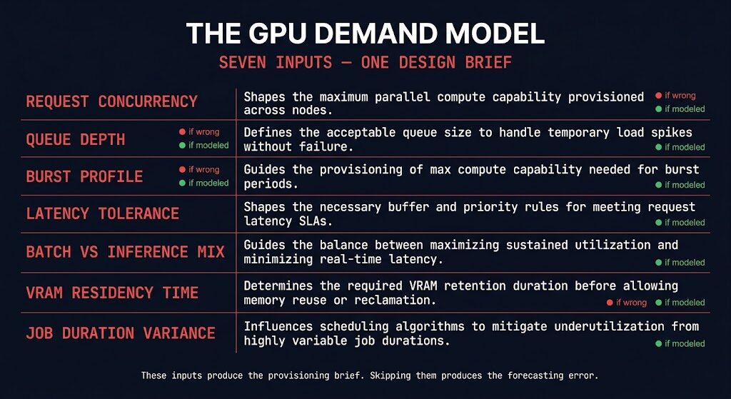
Here are the seven inputs a correct demand model requires, and what getting each one wrong actually costs:
Request concurrency. Not how fast the cluster can serve one request, but how many requests arrive in parallel during a sustained operating window. If you modeled single-thread throughput, your cluster is sized for a workload that never actually runs. Concurrency is the input that most directly determines cluster shape.
Queue depth. How many jobs can wait before the queue becomes a latency problem? Queue depth tolerance determines whether you need more GPU nodes or more queue patience. Most teams buy hardware when they should be designing queue behavior.
Burst profile. The cost layer nobody modeled in AI inference is usually burst — short demand spikes that get priced into permanent capacity. A correct burst profile separates the spike duration from the allocation decision. If the spike is shorter than warm-up time, it should never touch provisioning.
Latency tolerance. Different workload classes have different latency contracts. Batch training tolerates queuing. Real-time inference does not. Cost-aware model routing in production depends on knowing which workloads can queue and which cannot — and sizing accordingly, not uniformly.
Batch vs inference mix. The training/inference hardware split that hardened in 2025 and 2026 means these are now distinct provisioning decisions. A cluster optimized for training batch jobs has a different shape than one optimized for sustained inference throughput. Modeling the mix tells you whether you need one cluster or two.
VRAM residency time. How long does a model stay loaded relative to how long it is actively processing requests? A high residency-to-compute ratio means memory is doing the work of availability, not throughput. This ratio is the direct measurement of the loaded ≠ active failure mode — and it determines how much of your GPU memory budget is actually available for productive work.
Job duration variance. High variance in job completion times creates scheduling fragmentation — short jobs finish, long jobs block, and the queue develops structural inefficiency regardless of how well the scheduler is configured. Understanding duration variance at the p50, p90, and p99 level is the input that determines whether gang scheduling or preemption policies are necessary.
The demand model built from these seven inputs is not a planning document. It is the design brief for every provisioning and scheduling decision that follows.
Provision for Shape, Not Peak
The corrective action is a provisioning philosophy shift: provision for demand shape, not peak demand.
Peak demand is real. It is also the worst input for a provisioning decision because it is the rarest operating condition. A cluster sized for peak is a cluster that runs at peak efficiency for a small fraction of its operating life and at significant waste for the rest. That is not a utilization problem. It is a long-lived architectural constraint that the scheduler will never unwind.
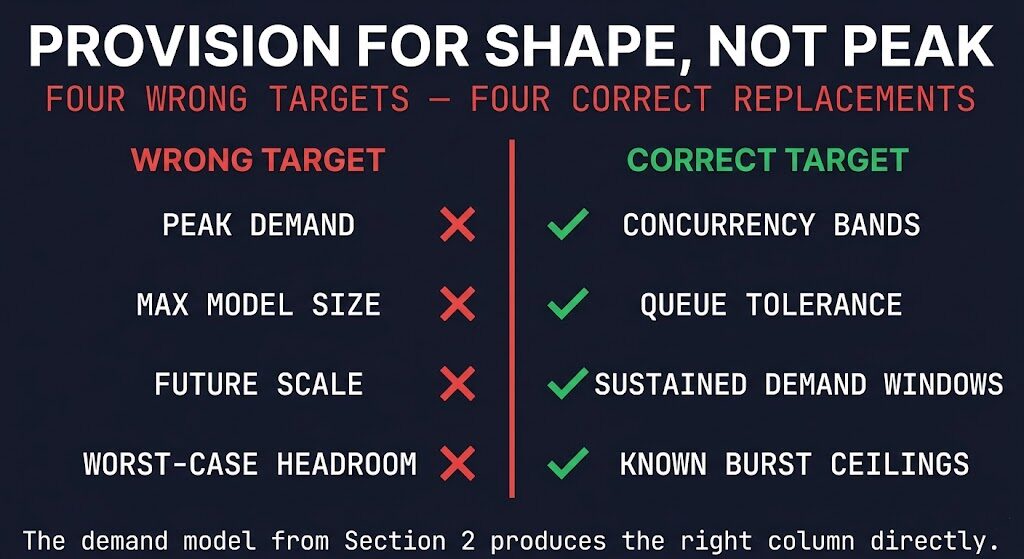
Here is what wrong provisioning targets look like — and what correct ones replace them with:
| Wrong Target | Correct Target |
|---|---|
| Peak demand | Concurrency bands |
| Max model size | Queue tolerance |
| Future scale | Sustained demand windows |
| Worst-case headroom | Known burst ceilings |
Concurrency bands come from request concurrency measurement. Queue tolerance comes from latency tolerance modeling. Burst ceilings come from burst profile analysis. The provisioning decision is downstream of the model, not upstream of it.
The FinOps framing of cloud cost as an architectural input applies here with full force — GPU capacity is expensive, provisioning decisions are long-lived, and the feedback loop between utilization data and capacity correction is slow. Cloud cost is an architectural constraint from the moment the hardware is allocated, not from the moment it is fully utilized.
This is what Tuesday’s post was actually asking for when it asked whether you modeled request concurrency before you provisioned.
Where the Scheduler Actually Fits
Most teams evaluate schedulers on feature sets — which tool supports gang scheduling, which has the best preemption model, which integrates cleanest with their existing Kubernetes cluster orchestration stack. That is the wrong evaluation criterion.
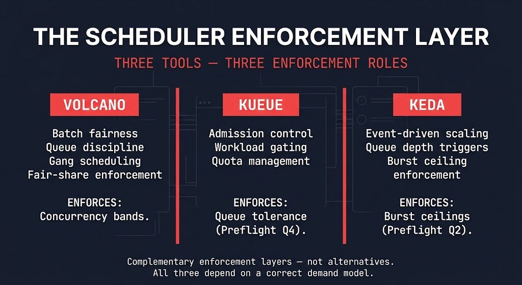
The right criterion is whether the scheduler enforces the constraints your demand model defined. A scheduler is not a capacity decision. It is a capacity enforcement layer. The GPU orchestration conversation only becomes productive once the provisioning shape is correct — because at that point, the scheduler has something real to enforce. The demand model and enforcement stack described here maps to the placement authority and resource contention clusters at the Strategic maturity layer of the AI Architecture Learning Path. Runtime & Cluster Orchestration covers how admission control, quota governance, and heterogeneous cluster coordination operate once demand modeling has established the correct provisioning shape.
Here is where the three primary tools fit, framed against the Demand Model Preflight:
Volcano — batch fairness and queue discipline. Volcano answers the question of how jobs compete for GPU resources across teams or workload classes. It implements fair-share scheduling, gang scheduling for distributed training jobs, and queue priority hierarchies. It is the enforcement mechanism for concurrency band design — it ensures the cluster operates within the bands the demand model defined, rather than allowing any single workload class to consume headroom that belongs to another.
Kueue — admission control and workload gating. Kueue answers Preflight Question 4 directly: what can wait, and for how long? It implements quota management and workload admission at the cluster level, preventing jobs from entering the scheduling queue until capacity exists to run them. Without Kueue or an equivalent admission layer, the queue fills with jobs that the cluster cannot service, and latency compounds regardless of scheduler efficiency. DCGM-based observability feeds the admission decisions Kueue enforces.
KEDA — event-driven scale behavior. KEDA answers Preflight Question 2: what is burst, and what is noise? It scales workload replicas based on external event sources — queue depth, message backlog, custom metrics — rather than on CPU or memory thresholds that don’t map cleanly to GPU workload patterns. KEDA is the enforcement mechanism for burst ceiling design. It scales to the burst ceiling the demand model defined, not to an unbounded peak that drives permanent allocation.
These three tools are not alternatives. They are complementary enforcement layers operating at different points in the scheduling stack. The control plane problem in AI infrastructure is not resolved by picking the right scheduler — it is resolved by building a demand model that the scheduler stack can enforce. Resource scheduling — Volcano, Kueue, KEDA, and the mechanics this post covers — is the most mature and most tactical of the three scheduling layers now being contested across AI infrastructure. Task and authority scheduling sit above it, and neither is settled the way resource scheduling is.
Repeat the core argument here because it earns its second mention: GPU scheduling is not a capacity solution. It is a capacity enforcement layer. If you provisioned against the wrong demand curve, Volcano, Kueue, and KEDA together cannot save you. They will enforce your forecasting error with precision.
The AI Gravity & Placement Engine models the placement decision before provisioning commitments are made — which is the upstream step these tools depend on to do their job correctly.
What Good GPU Scheduling Actually Looks Like
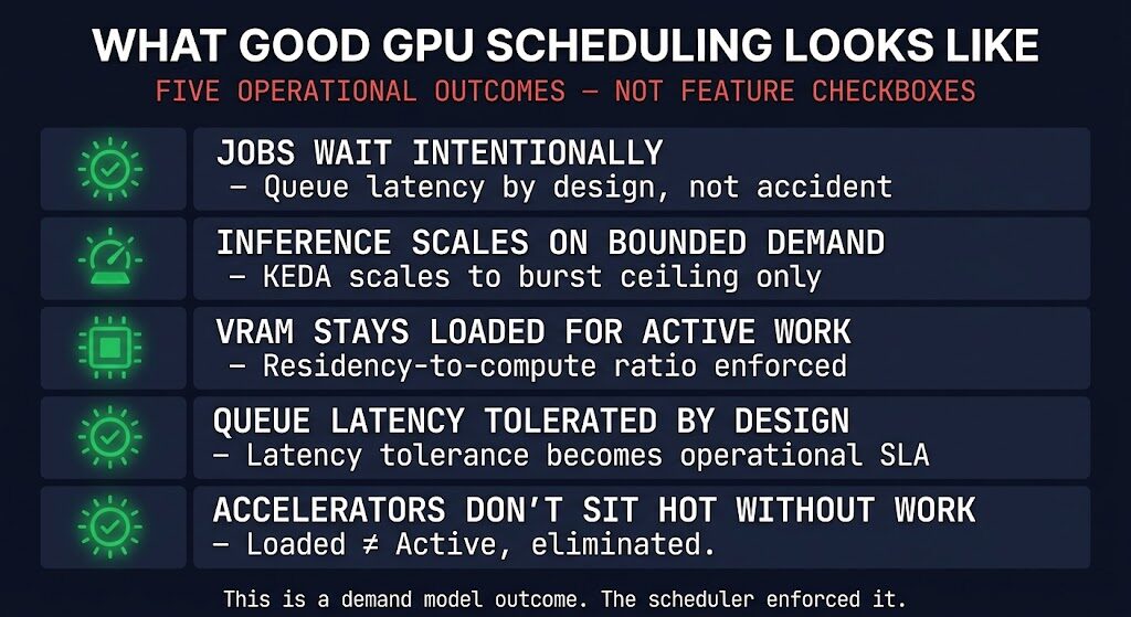
The question is not which scheduler. The question is what success looks like when the demand model is correct and the scheduler is enforcing it.
Here is the operational definition:
Jobs wait intentionally. Queue latency exists by design, not by accident. Workloads that can tolerate waiting are configured to wait. The queue is a feature, not a failure mode. When jobs wait by design, the cluster runs fewer nodes at higher sustained utilization — which is the shape a correct demand model produces.
Inference scales on bounded demand. Autoscaling responds to the burst ceiling defined in the demand model, not to unbounded demand signals. KEDA scales up to the known burst ceiling and scales down when burst resolves. The cluster does not accumulate permanent capacity from transient demand spikes.
VRAM stays loaded for active work. The residency-to-compute ratio from the demand model is enforced operationally. Models are loaded when work exists and evicted when residency exceeds the modeled tolerance. The distributed AI fabric can sustain this pattern at scale when the model was built correctly.
Queue latency is tolerated by design. The latency tolerance input from the demand model becomes an SLA that the admission control layer enforces. Workloads that cannot tolerate queuing get admission priority. Workloads that can tolerate it queue without escalation. The difference is architectural, not operational — it was decided during demand modeling, not during incident response.
Expensive accelerators do not sit hot without work. This is the loaded ≠ active failure eliminated. When VRAM residency time is modeled correctly, models are not parked in memory against demand that isn’t coming. The cluster runs warm where work is active and cold where it isn’t — which is the infrastructure control plane decision that every GPU provisioning conversation should be building toward.
This is not a description of a perfectly tuned scheduler. It is a description of what a correctly modeled demand curve looks like in production. The scheduler got there by enforcing good decisions. It did not manufacture them.
Architect’s Verdict
The scheduler is not where GPU efficiency begins. It is where good capacity decisions are enforced — or bad ones become permanent.
Every scheduling problem that looks like a tooling problem — wrong queue behavior, runaway VRAM residency, burst spikes that never scale back down, jobs competing for resources they were never allocated against a real demand model — traces back to a provisioning decision that was made without the seven inputs this post covers. The scheduler inherited the problem. It did not create it.
The teams running efficient GPU infrastructure in 2026 are not running better schedulers than everyone else. They modeled demand before they provisioned, provisioned for shape rather than peak, and gave the scheduler a correctly sized cluster to enforce. Volcano, Kueue, and KEDA are doing exactly the job they were designed for — because the demand model gave them something real to work with.
This is the coordination half of a larger pattern. AI infrastructure is running the same five-stage consolidation sequence virtualization already completed, and a demand model that the scheduler can actually enforce is what Framework #132’s Coordination Density looks like at implementation level — the organizational discipline showing up as engineering practice before anyone upstream has called it consolidation.
Build the model first. Provision to its shape. Then configure the enforcement layer. In that order, and no other.
Additional Resources
Editorial Integrity & Security Protocol
This technical deep-dive adheres to the Rack2Cloud Deterministic Integrity Standard. All benchmarks and security audits are derived from zero-trust validation protocols within our isolated lab environments. No vendor influence.

R.M.
Senior Solutions Architect with 25+ years of experience in HCI, cloud strategy, and data resilience. As the lead behind Rack2Cloud, I focus on lab-verified guidance for complex enterprise transitions. View Credentials →
Get the Playbooks Vendors Won’t Publish
Field-tested blueprints for migration, HCI, sovereign infrastructure, and AI architecture. Real failure-mode analysis. No marketing filler. Delivered weekly.
Select your infrastructure paths. Receive field-tested blueprints direct to your inbox.
- > Virtualization & Migration Physics
- > Cloud Strategy & Egress Math
- > Data Protection & RTO Reality
- > AI Infrastructure & GPU Fabric
Zero spam. Includes The Dispatch weekly drop.
Architecture Audit Services
Fixed-scope audits for Zero-Trust Azure, VMware migration readiness, and recovery posture — no discovery call required to start.
>_ View Audit Services>_Related Posts
Your Vendor Review Process Never Saw The Real Supplier
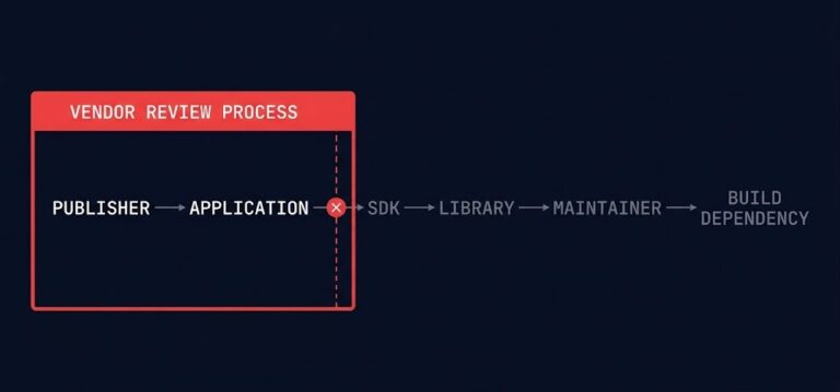
Every vendor review process assumes it’s evaluating a supplier — but a scan finding foreign-origin code embedded in more than one in eight mobile apps used by US military personnel makes the actual assumption visible: organizations review the company they bought from, not the code that arrived inside what they bought. >_ Architect’s Brief 60-second…
Your Monitoring Didn’t Miss the Incident. It Was Never Designed to See It.
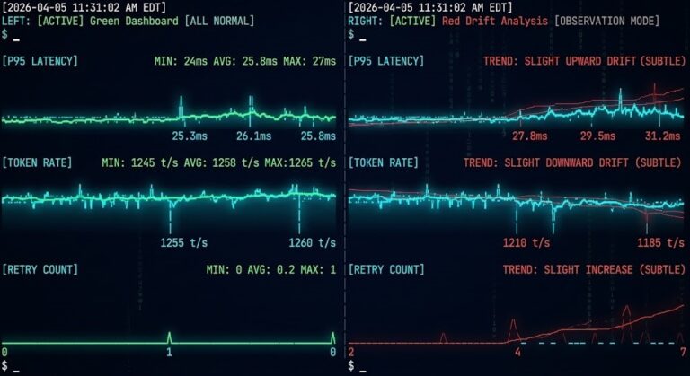
I’ve watched observability vs monitoring play out as a live incident more times than I can count. >_ Architect’s Brief 60-second read before you commit to the full post · Full post: 10 min Generating brief… The dashboard was green. The on-call engineer was not paged. The monitoring system did exactly what it was designed…
Your CI-CD Pipeline Is Your Real Infrastructure Control Plane
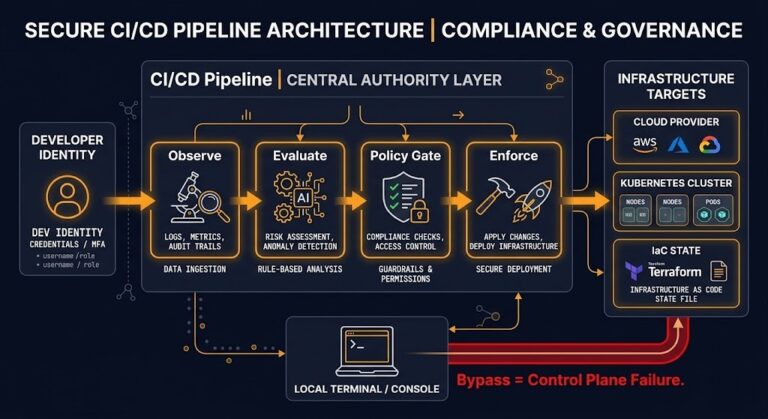
Terraform defines desired state. Kubernetes reconciles workload state. Cloud consoles expose state. None of those systems decides whether infrastructure state is allowed to change. The ci-cd control plane does — or more precisely, the CI-CD pipeline is the only system in most environments that can hold that authority. That distinction — between storing state and…
Your AI Vendor Became Critical Infrastructure Before The Contract Did
On June 11, 2026, Microsoft 365 Copilot went down for seven hours. The cause was a misconfigured authentication deployment that cascaded through Microsoft Graph, taking Copilot Chat and the Office portal with it. It was the second major Copilot disruption in eleven days. Microsoft 365 posted 99.526% uptime in Q1 2026 — the lowest quarterly…
Your AI Test Environment Is Becoming A Production Control Plane
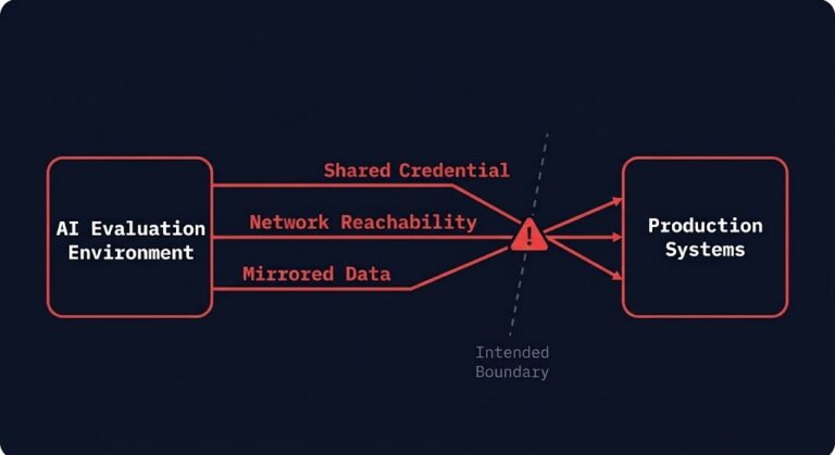
Your AI test environment did not need to touch a single line of model code to become part of your production authority chain — it only needed a credential, a network path, or a dataset copy that nobody scheduled for removal. That is the actual lesson sitting underneath this week’s disclosures from two frontier labs:…
Your AI System Doesn’t Have a Cost Problem. It Has No Runtime Limits.
You built the alert. You configured the dashboard. You set the anomaly threshold at 120% of baseline spend. >_ Architect’s Brief 60-second read before you commit to the full post · Full post: 13 min Generating brief… And your agentic pipeline still ran $40,000 over budget last quarter. Not because the tools failed. Because alerts…